Optimize FIS Parameters with K-Fold Cross-Validation

Data Overfitting in FIS Parameter Tuning

Data overfitting is a common problem in FIS parameter optimization. When overfitting occurs, the tuned FIS produces optimized results for the training data set but performs poorly for a test data set. Due to overtuning, the optimized FIS parameter values pick up noise from the training data set and lose the ability to generalize to new data sets. The difference between the training and test performance increases with the increased bias of the training data set.

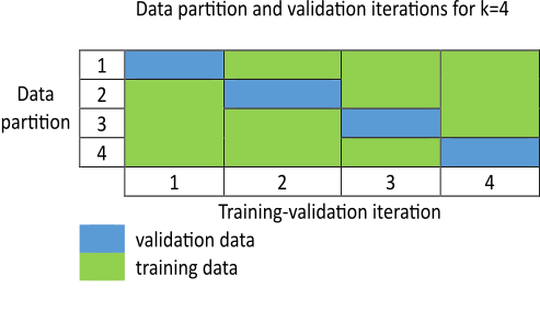
To overcome the data overfitting problem, you can stop a tuning process early based on an unbiased evaluation of the model using a separate validation data set. However, such a validation data set can also increase bias if it does not accurately represent the problem space. To overcome bias from the validation data set, a k-fold cross-validation approach is commonly used. Here, the training data is randomly shuffled and then divided into $\mathit{k}$ partitions, as shown in the following figure. For each training-validation iteration, you use a different partition for validation, and use the remaining data for testing. Therefore, you use each data partition once for validation and $\mathit{k}-1$ times for training.

Each training-validation iteration runs for $\mathit{n}$ cycles. However, an iteration can stop early and advance to the next iteration if an increase in the validation cost exceeds a predefined threshold value. The optimized model at the end of the ${\mathit{k}}^{\mathrm{th}}$ iteration is used as the output of the k-fold cross-validation process.

This example shows how using k-fold cross-validation with the tunefis function prevents data overfitting compared to parameter tuning that does not use k-fold cross-validation.

Tune FIS Without K-Fold Validation

This example describes a data overfitting problem for automobile fuel consumption prediction. It uses several automobile profile attributes to predict fuel consumption. The training data is available in the University of California at Irvine Machine Learning Repository and contains data collected from automobiles of various makes and models.

This example uses the following six input data attributes to predict the output data attribute MPG with a FIS.

Load the data using the loaddata utility function shown at the end of the example. This function creates training and test data sets.

[data,varName,trnX,trnY,testX,testY] = loadData;

Create an initial FIS based on the input and output data attributes using the constructFIS utility function.

fisin = constructFIS(data,varName);

Create an option set for tuning the FIS. The default option set uses GA for optimization.

options = tunefisOptions;

If you have Parallel Computing Toolbox™ software, you can improve the speed of the tuning process by setting options.UseParallel to true. If you do not have Parallel Computing Toolbox software, set options.UseParallel to false.

To demonstrate the data overfitting problem, this example uses a maximum of 100 generations to tune the rules.

options.MethodOptions.MaxGenerations = 100;

Tune the FIS using the specified tuning data and options. Tuning rules using the tunefis function takes several minutes. This example uses a flag, runtunefis, to either run the tunefis function or load pretrained results. To load the pretrained results, set runtunefis to false.

runtunefis = false;

To demonstrate the data overfitting problem, use the following performance measures:

In this example, use only rule parameter settings to tune the FIS.

Since GA optimization uses random search, to obtain reproducible results, initialize the random number generator to its default configuration.

if runtunefis    
    % Get rule parameter settings.
    [~,~,rule] = getTunableSettings(fisin);
    
    % Set default random number generator.    
    rng('default')    

    % Tune rule parameters.
    [outputFIS,optimData] = tunefis(fisin,rule,trnX,trnY,options);

    % Get the training error.
    trnErrNoKFold = optimData.tuningOutputs.fval
    
    % Calculate the test error.
    evalOptions = evalfisOptions("EmptyOutputFuzzySetMessage","none", ...
        "NoRuleFiredMessage","none","OutOfRangeInputValueMessage","none");
    actY = evalfis(outputFIS,testX,evalOptions);
    del = actY - testY;
    testErrNoKFold = sqrt(mean(del.^2))
    
    % Get the function count.
    fcnCountNoKFold = optimData.totalFcnCount
    
    save tuningWithoutKFoldValidation trnErrNoKFold testErrNoKFold fcnCountNoKFold
else
    % Load the pretrained results.
    results = load('tuningWithoutKFoldValidation.mat');
    trnErrNoKFold = results.trnErrNoKFold
    testErrNoKFold = results.testErrNoKFold
    fcnCountNoKFold = results.fcnCountNoKFold
end

trnErrNoKFold = 
2.4952

testErrNoKFold = 
2.8412

fcnCountNoKFold = 
19210

The higher value of the test error compared to the training error indicates that the trained FIS is more biased to the training data.

Tune FIS Parameters with K-Fold Validation

You can use k-fold cross-validation in FIS parameter optimization by setting options.KFoldValue to a value greater than or equal to 2. For this example, set the k-fold value to 4.

options.KFoldValue = 4;

To specify a tolerance value, used to stop the k-fold tuning process early, set the options.ValidationTolerance property. For this example, set the tolerance value to 0.02. This tolerance value configures the k-fold tuning process to stop if the current validation cost increases by more than 2% of the minimum validation cost found up to that point in the tuning process.

options.ValidationTolerance = 0.02;

For a noisy data set, you can compute a moving average of the validation cost by setting the options.ValidationWindowSize property to a value greater than 1. For this example, set the validation window size to 2.

options.ValidationWindowSize = 2;

Restrict the maximum number of generations in each tuning process to 25 so that the total number of generations in the 4-fold tuning process is the same as the previous case.

options.MethodOptions.MaxGenerations = 25;

Tune the FIS with k-fold validation.

if runtunefis    
    % Set default random number generator.
    rng('default')
    
    % Tune the FIS.
    [outputFIS,optimData] = tunefis(fisin,rule,trnX,trnY,options);
    
    % Get the training error.
    trnErrWithKFold = optimData.tuningOutputs(end).fval
    
    % Calculate the test error.
    actY = evalfis(outputFIS,testX,evalOptions);
    del = actY - testY;
    testErrWithKFold = sqrt(mean(del.^2))
    
    % Get the function count.
    fcnCountWithKFold = optimData.totalFcnCount
    
    save tuningWithKFoldValidation trnErrWithKFold testErrWithKFold fcnCountWithKFold
else
    % Load the pretrained results.
    results = load('tuningWithKFoldValidation.mat');
    trnErrWithKFold = results.trnErrWithKFold
    testErrWithKFold = results.testErrWithKFold
    fcnCountWithKFold = results.fcnCountWithKFold
end

trnErrWithKFold = 
2.7600

testErrWithKFold = 
2.9082

fcnCountWithKFold = 
5590

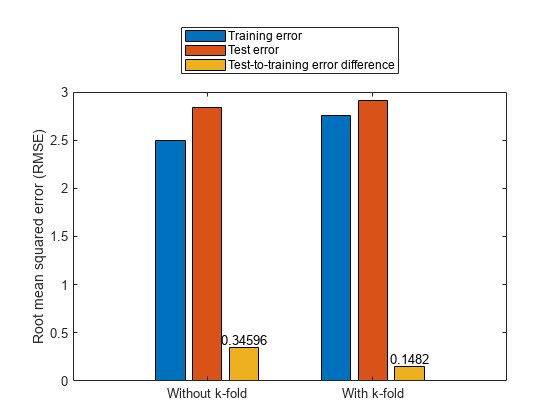
Plot the test-to-training error differences for training both with and without k-fold cases.

figure
cats = categorical({'Without k-fold','With k-fold'});
cats = reordercats(cats,{'Without k-fold','With k-fold'});
data = [trnErrNoKFold testErrNoKFold testErrNoKFold-trnErrNoKFold; ...
    trnErrWithKFold testErrWithKFold testErrWithKFold-trnErrWithKFold];
b = bar(cats,data);
ylabel('Root mean squared error (RMSE)')
text(b(3).XEndPoints,b(3).YEndPoints,string(b(3).YData),...
    'HorizontalAlignment','center','VerticalAlignment','bottom')
legend('Training error','Test error',...
    'Test-to-training error difference','Location','northoutside')

The test error performance is similar in both cases. However, the difference in the training and test errors with k-fold validation is less than without k-fold validation. Therefore, the k-fold validation reduces the bias of the training data and produces better generalized FIS parameter values. The total function count during k-fold validation is fewer than the count without k-fold validation.

disp(table(fcnCountNoKFold,fcnCountWithKFold, ...
    'VariableNames',["Without k-fold" "With k-fold"], ...
    'RowName',"Function counts"))

                       Without k-fold    With k-fold
                       ______________    ___________

    Function counts        19210            5590    

Therefore, k-fold validation reduces the number of generations in each GA optimization cycle, reducing FIS parameter overfitting. The overall k-fold validation results can be further improved by experimenting with different k-fold, tolerance, and window size values.

In general, use the following process for FIS parameter optimization with k-fold validation:

High values of tolerance, window size, and k-fold value introduce data overfitting in the optimized FIS parameter values. Therefore, use smaller values to achieve your desired tuning performance.

Local Functions

function [data,varName,trnX,trnY,testX,testY] = loadData

% Load the data. Each row of the dataset obtained from the repository represents 
% a different automobile profile. Data contains 7 columns, where the first six 
% columns contain the following input attributes.
%   - Number of cylinders
%   - Displacement
%   - Horsepower
%   - Weight
%   - Acceleration
%   - Model year
% The seventh column contains the output attribute, MPG.
[data,name] = loadGasData;

% Remove leading and trailing whitespace from the attribute names.
varName = strtrim(string(name));

% Create input and output data sets.
n = size(data,2);
x = data(:,1:n-1);
y = data(:,n);

% Create training and test data sets.
trnX = x(1:2:end,:);
trnY = y(1:2:end,:);
testX = x(2:2:end,:);
testY = y(2:2:end,:);

end

function fisin = constructFIS(data,varName)

% Create a Sugeno FIS.
fisin = sugfis;

% Add input and output variables to the FIS, where each variable represents
% one of the data attributes. For each variable, use the corresponding
% attribute name and range. To reduce the number of rules, use two MFs for
% each input variable, which results in 2^6=64 input MF combinations.
% Therefore, the FIS uses a maximum of 64 rules corresponding to the input
% MF combinations. Both input and output variables use default triangular
% MFs, which are uniformly distributed over the variable ranges.
dataRange = [min(data)' max(data)'];
numINputs = size(data,2)-1;
numInputMFs = 2;
numOutputMFs = numInputMFs^numINputs;
for i = 1:numINputs
    fisin = addInput(fisin,dataRange(i,:),...
        'Name',varName(i),'NumMFs',numInputMFs);
end

% To improve data generalization, use 64 MFs for the output variable.
% Doing so allows the FIS to use a different output MF for each rule.
fisin = addOutput(fisin,dataRange(end,:),...
    'Name',varName(end),'NumMFs',numOutputMFs);
fisin.Rules = repmat(fisrule,[1 numOutputMFs]);

end