Train ANFIS Systems at the Command Line
This example shows how to create, train, and test an adaptive neuro-fuzzy inference system (ANFIS) at the MATLAB® command line. For more information on:
Neuro-adaptive fuzzy systems, see Neuro-Adaptive Learning and ANFIS.
Training ANFIS systems using Fuzzy Logic Designer, see Train ANFIS Systems Using Fuzzy Logic Designer.
Load Example Data
Training and validating ANFIS models requires existing data. Import the training data sets to the MATLAB workspace. Each data set has one input and one output.
load anfisTrainingDataThe data for this example includes two training data sets and two validation data sets.
Training data set 1 with input data
trnInput1and output datatrnOutput1Training data set 2 with input data
trnInput2and output datatrnOutput2Validation data set 1 with input data
valInput1and output datavalOutput1Validation data set 2 with input data
valInput2and output datavalOutput2
Specify FIS Structure
To train an ANFIS model, you must first define the FIS structure. The system you define must be a Sugeno system with the following properties:
Single output
Weighted average defuzzification
First or zeroth order system; that is, all output membership functions must be the same type, either linear or constant.
No rule sharing. Different rules cannot use the same output membership function; that is, the number of output membership functions must equal the number of rules.
Unity weight for each rule.
No custom membership functions or defuzzification methods.
For this example, generate a FIS based on your training data using the genfis function. Alternatively, you can programmatically construct a sugfis object.
Specify option for generating a FIS using grid partitioning. Use four membership functions for the input variable.
genOpt = genfisOptions("GridPartition");
genOpt.NumMembershipFunctions = 4;
Create the FIS structure based on the first set of training data.
inFIS = genfis(trnInput1,trnOutput1,genOpt);
Specify Training Options
To specify tuning options, create a tunefisOptions object, specifying the ANFIS tuning method.
opt = tunefisOptions(Method="anfis");To configure ANFIS tuning options, use the MethodOptions property of the options object. For this example:
Set the maximum number of training epochs to 40.
Keep the default error stopping condition of
0. Doing so indicates that the training does not stop until the maximum number of training epochs complete.
For more information on the ANFIS tuning options, see ANFISOptions Properties.
opt.MethodOptions.EpochNumber = 40;
To prevent overfitting, specify validation data for training.
opt.MethodOptions.ValidationData = [valInput1 valOutput1];
Train FIS
To train your FIS, first obtain the tunable settings for the initial FIS structure.
[in,out] = getTunableSettings(inFIS);
ANFIS training does not support customized tunable settings. Therefore, do not modify the tunable settings objects and pass them directly to the tunefis function.
Tune the FIS using the first set of training data and the specified training options.
[outFIS,summary] = tunefis(inFIS,[in;out],trnInput1,trnOutput1,opt);
ANFIS info:
	Number of nodes: 20
	Number of linear parameters: 8
	Number of nonlinear parameters: 12
	Total number of parameters: 20
	Number of training data pairs: 25
	Number of checking data pairs: 26
	Number of fuzzy rules: 4


Start training ANFIS ...

1 	 0.138854 	 0.148022
2 	 0.137056 	 0.147738
3 	 0.135673 	 0.14769
4 	 0.134574 	 0.14764
Step size increases to 0.011000 after epoch 5.
5 	 0.133616 	 0.14737
6 	 0.132755 	 0.146922
7 	 0.131887 	 0.146268
8 	 0.131071 	 0.145404
Step size increases to 0.012100 after epoch 9.
9 	 0.130275 	 0.144336
10 	 0.129473 	 0.143094
11 	 0.128558 	 0.14161
12 	 0.127587 	 0.140069
Step size increases to 0.013310 after epoch 13.
13 	 0.126535 	 0.138586
14 	 0.125371 	 0.137209
15 	 0.123916 	 0.135963
16 	 0.122211 	 0.135026
Step size increases to 0.014641 after epoch 17.
17 	 0.120184 	 0.134579
18 	 0.117772 	 0.134654
19 	 0.114644 	 0.135497
20 	 0.111056 	 0.137048
Step size increases to 0.016105 after epoch 21.
21 	 0.107128 	 0.139065
22 	 0.103046 	 0.141098
23 	 0.0986361 	 0.143063
24 	 0.0945757 	 0.144691
Step size increases to 0.017716 after epoch 25.
25 	 0.0910926 	 0.146156
26 	 0.088364 	 0.147012
27 	 0.0863009 	 0.150075
28 	 0.0902995 	 0.137683
29 	 0.0859508 	 0.153196
30 	 0.0894718 	 0.137312
Step size decreases to 0.015944 after epoch 31.
31 	 0.0855071 	 0.153066
32 	 0.0888458 	 0.137204
33 	 0.0844305 	 0.151175
34 	 0.0882056 	 0.137509
Step size decreases to 0.014350 after epoch 35.
35 	 0.0841874 	 0.151597
36 	 0.0878093 	 0.137471
37 	 0.0835071 	 0.149968
38 	 0.0873794 	 0.137848
Step size decreases to 0.012915 after epoch 39.
39 	 0.0833853 	 0.150399
40 	 0.0871196 	 0.137795

Designated epoch number reached. ANFIS training completed at epoch 40.

Minimal training RMSE = 0.0833853
Minimal checking RMSE = 0.134579
The outFIS model is the FIS corresponding to the minimum training error. This FIS is potentially overfit to the training data.
The summary structure has a tuningOutputs field that contains the following additional training results:
trainError— Training error values for each training epochstepSize— Step size for each training epochchkFIS— Trained FIS that corresponds to the minimum validation errorchkError— Validation error values for each training epoch
Plot the training error and validation error.
trnError = summary.tuningOutputs.trainError;
valError = summary.tuningOutputs.chkError;

x = [1:40]';
plot(x,trnError,"-*",x,valError,"-o")
xlabel("Epoch")
ylabel("Error")
legend("Training error","Validation error",Location="southwest")
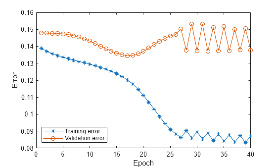
The validation error decreases up to a certain point in the training, and then it increases. This increase occurs at the point where the training starts overfitting the training data.
Obtain the FIS that corresponds to this overfitting inflection point. This minimum validation error shows that this FIS achieved the best generalization beyond the training data.
tunedFIS = summary.tuningOutputs.chkFIS;
Compare FIS Output to Training Data
To validate the performance of the tuned model, evaluate the FIS using the input training data and compare the resulting output to the output training data.
tunedOutput = evalfis(tunedFIS,trnInput1);

x = trnInput1;
plot(x,trnOutput1,"-*",x,tunedOutput,"-o")
legend("Training Data","ANFIS Output",Location="northwest")
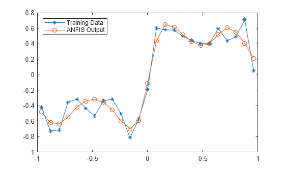
The FIS output correlates well with the reference output.
Importance of Validation Data
It is important to have validation data that fully represents the features of the data the FIS is intended to model. If your validation data is significantly different from your training data and does not cover the same data features to model as the training data, then the training results will be poor.
For example, train an ANFIS system data with significantly different training and validation sets.
opt.MethodOptions.ValidationData = [valInput2 valOutput2];
[outFIS2,summary2] = tunefis(inFIS,[in;out],trnInput2,trnOutput2,opt);
ANFIS info:
	Number of nodes: 20
	Number of linear parameters: 8
	Number of nonlinear parameters: 12
	Total number of parameters: 20
	Number of training data pairs: 25
	Number of checking data pairs: 26
	Number of fuzzy rules: 4


Start training ANFIS ...

1 	 0.354303 	 0.629968
2 	 0.352383 	 0.632459
3 	 0.350503 	 0.635013
4 	 0.348658 	 0.637653
Step size increases to 0.011000 after epoch 5.
5 	 0.346847 	 0.640402
6 	 0.34507 	 0.64328
7 	 0.34316 	 0.646619
8 	 0.341297 	 0.650151
Step size increases to 0.012100 after epoch 9.
9 	 0.33948 	 0.653889
10 	 0.337703 	 0.657846
11 	 0.335771 	 0.66247
12 	 0.333818 	 0.667375
Step size increases to 0.013310 after epoch 13.
13 	 0.331764 	 0.672555
14 	 0.329498 	 0.677997
15 	 0.326609 	 0.684333
16 	 0.323134 	 0.691077
Step size increases to 0.014641 after epoch 17.
17 	 0.318907 	 0.698338
18 	 0.313787 	 0.706176
19 	 0.30704 	 0.715356
20 	 0.299254 	 0.724367
Step size increases to 0.016105 after epoch 21.
21 	 0.290974 	 0.731522
22 	 0.283081 	 0.734172
23 	 0.275529 	 0.730123
24 	 0.269547 	 0.721959
Step size increases to 0.017716 after epoch 25.
25 	 0.264992 	 0.716449
26 	 0.263253 	 0.708297
27 	 0.266379 	 0.713912
28 	 0.262273 	 0.706052
29 	 0.264892 	 0.713268
Step size decreases to 0.015944 after epoch 30.
30 	 0.261561 	 0.704701
31 	 0.263862 	 0.712828
32 	 0.259939 	 0.705403
33 	 0.262939 	 0.71243
Step size decreases to 0.014350 after epoch 34.
34 	 0.259517 	 0.70457
35 	 0.262258 	 0.712199
36 	 0.258346 	 0.705435
37 	 0.2616 	 0.711973
Step size decreases to 0.012915 after epoch 38.
38 	 0.258076 	 0.704897
39 	 0.261096 	 0.711884
40 	 0.257239 	 0.705789

Designated epoch number reached. ANFIS training completed at epoch 40.

Minimal training RMSE = 0.257239
Minimal checking RMSE = 0.629968
Plot the training error and validation error.
trnError2 = summary2.tuningOutputs.trainError;
valError2 = summary2.tuningOutputs.chkError;

x = [1:40]';
plot(x,trnError2,"-*",x,valError2,"-o")
xlabel("Epoch")
ylabel("Error")
legend("Training error","Validation error",Location="southwest")
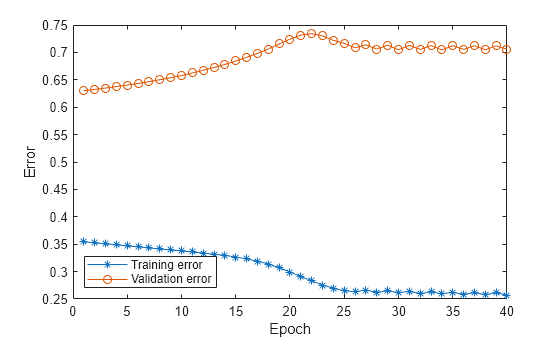
In this case, the validation error is large, with the minimum occurring in the first epoch. Therefore, the trained FIS does not sufficiently capture the features of the validation data set. It is important to know the features of your data set well when you select your training and validation data. When you do not know the features of your data, you can analyze the validation error plots to see whether or not the validation data performed sufficiently well with the trained model.
To verify the poor training results, test the trained FIS model against the validation data.
tunedFIS2 = summary2.tuningOutputs.chkFIS;

tunedOutput2 = evalfis(tunedFIS2,valInput2);

x = valInput2;
plot(x,valOutput2,"-*",x,tunedOutput2,"-o")
legend("Training Data","ANFIS Output",Location="northwest")
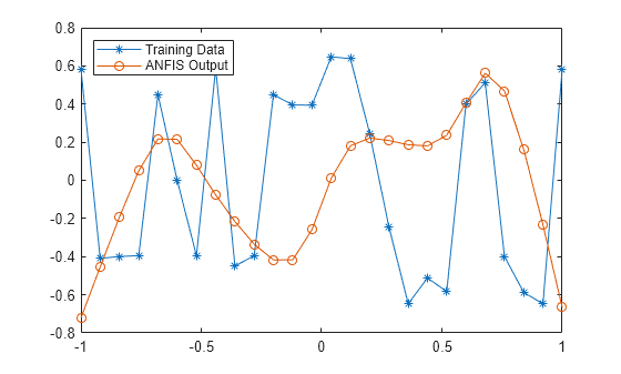
As expected, there are significant differences between the validation data output values and the FIS output.
See Also
tunefis | tunefisOptions | genfis