Tune FIS Tree Using Fuzzy Logic Designer
This example shows how to interactively tune membership function (MF) and rule parameters of FIS tree using Fuzzy Logic Designer. This example uses particle swarm and pattern search optimization, which require Global Optimization Toolbox software.
For more information on FIS trees, see FIS Trees.
For an example that programmatically tunes a FIS tree using the same data, see Tune FIS Tree at the Command Line.
For an example that interactively tunes a FIS using the same data, see Tune Fuzzy Inference System Using Fuzzy Logic Designer.
Load Example Data
This example trains a FIS using automobile fuel consumption data. The goal is for the FIS to predict fuel consumption in miles per gallon (MPG) using several automobile profile attributes. The training data is available in the University of California at Irvine Machine Learning Repository and contains data collected from automobiles of various makes and models.
This example uses the following six input data attributes to predict the output data attribute MPG with a FIS:
Number of cylinders
Displacement
Horsepower
Weight
Acceleration
Model year
Load the data. Each row of the data set obtained from the repository represents a different automobile profile.
[data,name] = loadGasData;
data contains seven columns, where the first six columns contain the input attribute values. The final column contains the predicted MPG output. Split data into input and output data sets, X and Y, respectively.
X = data(:,1:6);
Y = data(:,7);
Partition the input and output data sets into training data (odd-indexed samples) and validation data (even-indexed samples).
trnX = X(1:2:end,:); % Training input data set
trnY = Y(1:2:end,:); % Training output data set
vldX = X(2:2:end,:); % Validation input data set
vldY = Y(2:2:end,:); % Validation output data set
The FIS tree structure that you create in this example uses a different input order than the original data. Rearrange the training and validation input data to use the new order.
inputOrders1 = [4 6 2 5 3 1];
trnX = trnX(:,inputOrders1);
vldX = vldX(:,inputOrders1);
Initial FIS Tree Structure
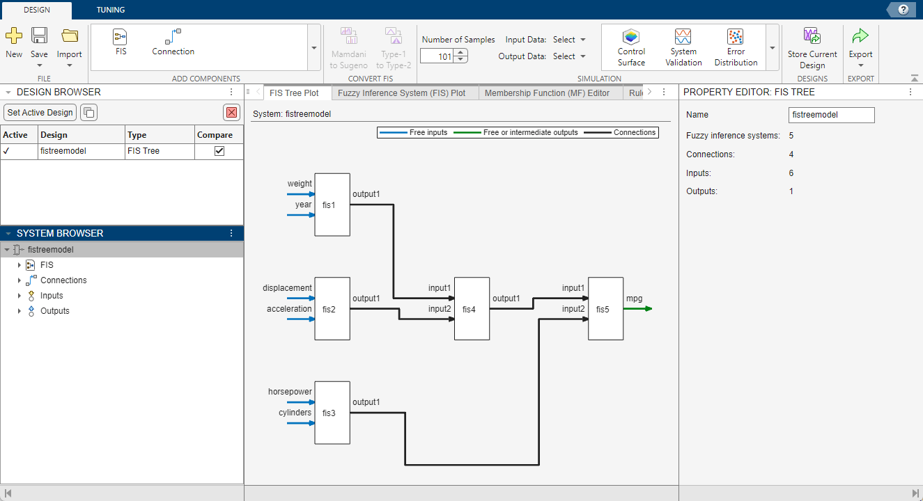
To train a FIS tree, you must first create an initial FIS tree structure. For this example, you use the following FIS tree.

Load the initial structure.
load mpgInitialFISTreeThis FIS tree was created using the following steps:
Rank the input attributes based on their correlations with the output attribute.
Create multiple FIS objects using the ranked input attributes.
Construct a FIS tree from the FIS objects.
For more information on creating this FIS tree structure, see Tune FIS Tree at the Command Line.
Define Initial FIS Tree Structure
The first step of the tuning process is to define the initial structure of your FIS tree. To define this structure, specify:
Component FIS objects, specifying the following for each FIS:
Input and output variables with defined ranges
Initial membership functions for each variable
Initial rule base (optional)
Connections between FIS objects
Output configuration for the FIS tree
To create your FIS in the app, you can:
Manually build a FIS tree. For an example, see Build FIS Tree Using Fuzzy Logic Designer.
Create a FIS tree at the command line and import It into the app.
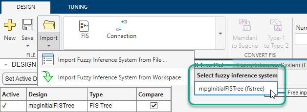
For this example, open Fuzzy Logic Designer and import the
mpgInitialFISTree system from the MATLAB® workspace.
fuzzyLogicDesigner(mpgInitialFISTree)
Import Training Data
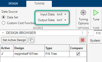
To select input and output data for tuning, on the Tuning tab:
In the Input Data list, under Workspace Data Sets, select trnX.
In the Output Data list, under Workspace Data Sets, select trnY.
Tune FIS Tree
Tuning is performed in two steps.
Learn the rule base for each FIS while keeping the input and output MF parameters constant.
Tune the parameters of the input/output MFs and rules for each FIS.
The first step is less computationally expensive due to the small number of rule parameters, and it quickly converges to a fuzzy rule base during training. In the second step, using the rule base from the first step as an initial condition provides fast convergence of the parameter tuning process.
Learn Rules
To learn the rules for your FIS, first specify the tuning options. Click Tuning Options.
In the Tuning Options dialog box, configure the following tuning options:
In the Optimization Type section, select Learning.
In the Method list, select
Particle
                                swarm
. Particle swarm optimization is a global optimization method. Such methods perform better in large parameter tuning ranges as compared to local optimization methods.Set the maximum number of optimization iterations to
50.Clear the Use default method options parameter.
Under Method Options: Particle swarm, in the leftmost list, select
Run time
                                        limits
. By default, the next list showsMax Iterations.In the text box, enter
20.
Set the maximum number of rules to generate for each FIS during learning. Clear the auto parameter and set the Max number of rules option to
4.For reproducible results, set the Random number seed parameter to the
Initialize Mersenne Twister generatoroption.Keep the remaining training options at their default values.

Click OK.
To only learn rules without modifying the MF parameters, you must disable the input and output tunable parameter settings for all FIS objects.
In the System Browser, under FIS,
select fis1.
In the Tunable Parameters pane, click Tune None for both the input and output tables.
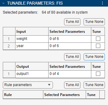
Repeat this process for the remaining FIS objects, fis2,
fis3, fis4, and
fis5.
To train the FIS, on the Tuning tab, click Tune. For this example, learning rules takes several minutes.
The Tune tab shows the training progress.
The Convergence Plot document plots the optimization cost (training error) after each epoch for both the training and validation data.
The Convergence Results document shows the algorithm-specific tuning progress.
The following figure shows the completed training process. The training error decreases throughout the tuning process. The tuning stops after the maximum number of iterations is reached.

The final root mean squared error (RMSE) cost value for the tuned FIS tree is 3.271 MPG.
To accept the training results, click Accept.
The app adds the tuned FIS tree mpgInitialFISTree_tuned to
the Design Browser and sets this FIS tree as the active
design.
Select the mpgInitialFISTree_tuned row in the
Design Browser. Click the FIS tree name and rename it
to fistree_learned.

To validate the performance of the tuned FIS tree, compare its performance to the validation data.
To select validation data, on the Design tab:
In the Input Data list, under Workspace Data Sets, select vldX.
In the Output Data list, under Workspace Data Sets, select vldY.

To ensure that the first untuned FIS tree is not included in any system validation, in the Design Browser, clear the corresponding entry in the Compare column.

On the Design tab, in the Simulation gallery, click System Validation.
The System Validation document shows the input values, reference output values, and FIS tree output values.
To view just the reference and FIS tree output values, click Unselect All for the Reference Inputs table.
To view the error between the reference and FIS tree output values, select Prediction errors.
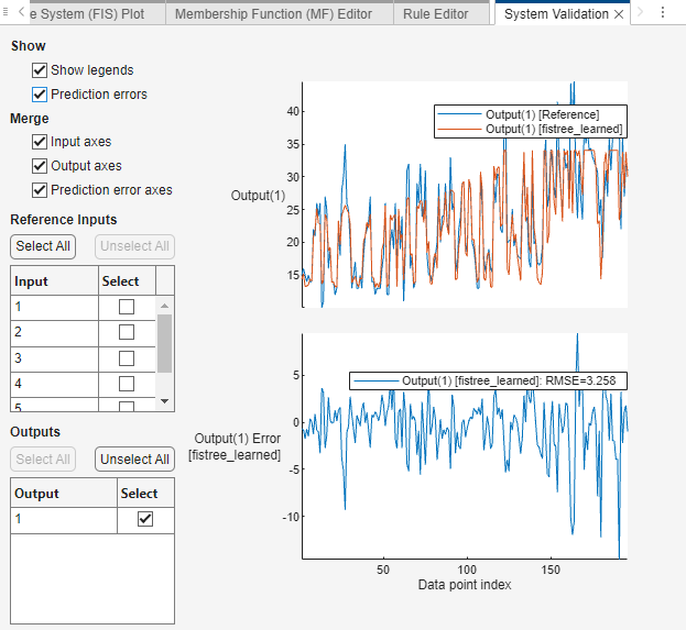
The FIS tree output tracks the reference output well.
The bottom plot shows the output error. The legend for this plot displays an RMSE of 3.258 MPG for the validation data, which is comparable to the RMSE for the training data.
Tune All Parameters
To further improve the FIS performance, you can tune the MF and rule
parameters of fistree_learned. To do so, first specify the
tuning options.
On the Tuning tab, click Tuning Options.
In the Tuning Options dialog box, configure the following tuning options:
In the Optimization Type section, select Tuning.
In the Method list, select
Pattern
                                search
, which is a local optimization method that converges quickly for the parameter tuning.Set the maximum number of optimization iterations to
75.Under Method Options: Pattern search, in the leftmost list, select
Run time limits.In the next list, select
Max Iterations.In the text box, enter
75.
To improve the pattern search results, use a complete poll.
Under Method Options: Pattern search, click +. The app adds a new option row.
In this row, in the leftmost list, select
Poll
                                        settings
In the next list, select
Do a complete poll.Select the checkbox.
Keep the remaining training options at their previous values.

Click OK.
To tune the MF and rule parameters, you must ensure that the corresponding tunable parameter settings are enabled.
In the System Browser, select
fis1.In the Tunable Parameters pane, click Tune All for both the input and output tables.
In the rule table, all the rule parameters are already selected.
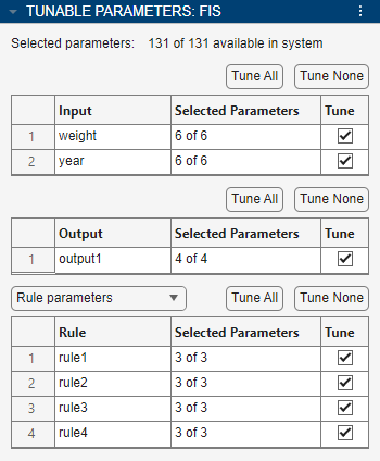
Repeat this process for the remaining FIS objects, fis2,
fis3, fis4, and
fis5.
To train the FIS, on the Tuning tab, click Tune. For this example, tuning parameters can take several minutes.
The following figure shows the completed training process. The training error decreases throughout the tuning process. The training stops after the maximum number of iterations is reached.

The final root mean squared error (RMSE) cost value for the tuned FIS is 3.011 MPG.
To accept the training results, click Accept.
The app adds the tuned FIS tree fistree_learned_tuned to
the Design Browser and sets this FIS tree as the active
design.
Rename this FIS tree to fistree_tuned.
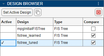
Open the System Validation document. The plots update to
show the validation results for fistree_tuned.
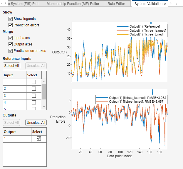
The results are similar to the results for fistree_learned.
In the Prediction Errors plot, the RMSE for
fistree_tuned is 3.057 MPG. Tuning the MF and rule
parameters has improved the performance of the tuned FIS.
Analyze Intermediate Data
To gain insight into the operation of your FIS tree, you can add the outputs of
the component FIS objects as outputs of your FIS tree. For this example, examine how
the outputs of fis1, fis2, and
fis3 correlate with the output validation data.
First, since you are analyzing the behavior of fistree_tuned,
remove the fistree_learned output from the System
Validation plots. To do so, in the Design
Browser, clear the entry in the Compare column
for fis_learned.
To compare FIS tree outputs with validation data, the number of FIS tree outputs
must match the number of outputs in the validation output data, which for this
example is one. To configure the FIS tree outputs, in the System
Browser, under fistree_tuned, click
Outputs.
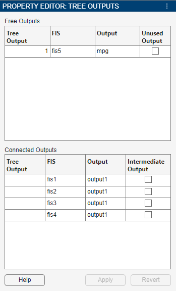
To make the output of fis1 the only output of the FIS tree, in
the Property Editor:
Disable the output of
fis5. In the Free Outputs table, select the entry in the Unused Output column forfis5.Configure the output of
fis1as a FIS tree output. In the Connected Outputs table, select the entry in the Intermediate Output column forfis1.
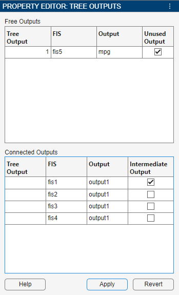
Click Apply.
In the System Validation document, clear the Prediction errors checkbox.
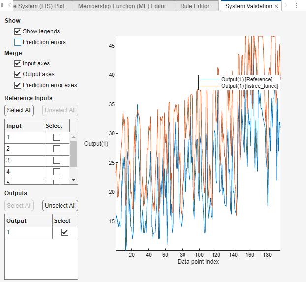
Repeat this process to view the output behavior for
fis2.
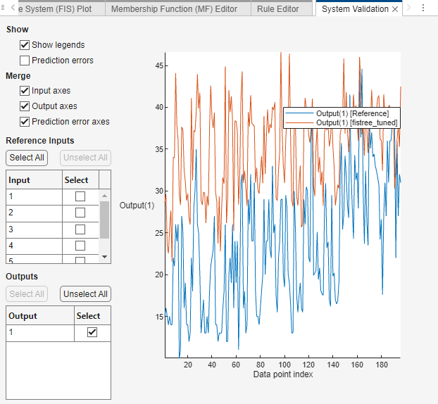
Repeat this process to view the output behavior for
fis3.
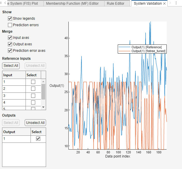
The outputs of fis1, fis2, and
fis3 all correlate with the output validation data. The
correlation of fis1 appears to be strongest, followed by
fis3.
To validate this analysis, you can export the system validation simulation results to the MATLAB workspace for further analysis. For more information on exporting simulation results, see Export Simulation Data. For an example correlation analysis, see the command-line tuning example Tune FIS Tree at the Command Line
After analyzing the intermediate outputs, reset the FIS output configuration. In
the Property Editor enable the output fis5
as a FIS tree output and clear the Intermediate Output value
the connected outputs.
Simplify and Retrain FIS Tree
For this example, to see if you can get comparable performance for a simplified
FIS tree, remove fis2 and fis4 from the
original FIS structure and retune the FIS tree.
To do so, first open a new instance of Fuzzy Logic Designer with the
original FIS tree structure. On the Design tab, under Open > Open Fuzzy Inference System from Workspace, select mpgInitialFISTree.
To remove fis2, in the System Browser,
under FIS, right-click fis2 and select
Delete. When you delete a FIS object from your FIS
tree, any connections to that FIS object are also removed.
Similarly, remove fis4.
Connect the output of fis1 to the first input of
fis5.
The following figure shows the resulting FIS tree configuration.

To learn rules, disable parameter tuning for fis1,
fis3, and fis5. In the System
Browser, under FIS, select each FIS individually
and, in the Tunable Parameters pane, click Tune
None for both the input and output tables.
On the Tuning tab, select the simplified four-input training data:
In the Input Data list, select simpleTrnX.
In the Output Data list, select trnY.
Click Tuning Options. In the Tuning Options dialog box, configure the same rule-learning options that you used previously, as shown in the following figure.

Click Tune.

The RMSE for this learning step is 3.368, which is similar to the result from the original rule learning step.
Accept the training result and rename the resulting FIS tree design to
mpgsimple_learned.
To tune the rule and MF parameters, configure the same parameter-tuning options that you used previously, as shown in the following figure.

Click Tune.
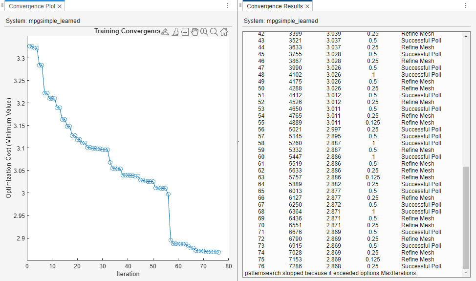
The RMSE for this learning step is 2.868, which is lower than the result from the original rule learning step.
Accept the training result and rename the resulting FIS tree design to
mpgsimple_tuned.
To validate the final tuned system, first select the Compare
checkbox for the mpgsimple_tuned system in the Design
Browser, and clear the Compare checkbox for all
the other designs.
On the Design tab:
In the Input Data list, select simpleVldX.
In the Output Data list, select vldY.
Open the System Validation document.

The RMSE for the validation data is 3.014, which is similar to the result from the original rule learning step.
Export Tuned FIS Tree
To save your FIS tree for further analysis and development, you can either export it to the MATLAB workspace or save it to a FIS file. For this example, export both the simplified tuned FIS tree to the MATLAB workspace.
On the Design tab, under Export, select Export Fuzzy Inference System to Workspace.
In the Export Fuzzy Inference System to Workspace dialog box, in the
Export column, select the checkbox for
mpgsimple_tuned.
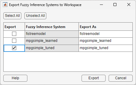
Click Export.