Generate GPU Code for Fog Rectification Algorithm
This example shows how to generate a CUDA® MEX function for a fog rectification algorithm. The entry-point function takes a foggy image as input and produces a defogged image.
Third-Party Prerequisites
Required
This example generates CUDA MEX and requires a CUDA-enabled NVIDIA® GPU and compatible driver. For half-precision code generation, the GPU must have a minimum compute capability of 6.0.
Optional
For non-MEX builds such as static, dynamic libraries or executables, this example has the following additional requirements.
NVIDIA toolkit.
Environment variables for the compilers and libraries. For more information, see Third-Party Hardware and Setting Up the Prerequisite Products.
Verify GPU Environment
To verify that the compilers and libraries necessary for running this example are set up correctly, use the coder.checkGpuInstall function.
envCfg = coder.gpuEnvConfig('host');
envCfg.BasicCodegen = 1;
envCfg.Quiet = 1;
coder.checkGpuInstall(envCfg);
The fog_rectification Entry-Point Function
The fog_rectification.m entry-point function takes a foggy image as input and returns a defogged image.
type fog_rectificationfunction [out] = fog_rectification(input) %#codegen
%
% Copyright 2017-2023 The MathWorks, Inc.
coder.gpu.kernelfun;
% restoreOut is used to store the output of restoration
restoreOut = zeros(size(input),"double");
% Changing the precision level of input image to double
input = double(input)./255;
%% Dark channel Estimation from input
darkChannel = min(input,[],3);
% diff_im is used as input and output variable for anisotropic
% diffusion
diff_im = 0.9*darkChannel;
num_iter = 3;
% 2D convolution mask for Anisotropic diffusion
hN = [0.0625 0.1250 0.0625; 0.1250 0.2500 0.1250;
0.0625 0.1250 0.0625];
hN = double(hN);
%% Refine dark channel using Anisotropic diffusion.
for t = 1:num_iter
diff_im = conv2(diff_im,hN,"same");
end
%% Reduction with min
diff_im = min(darkChannel,diff_im);
diff_im = 0.6*diff_im ;
%% Parallel element-wise math to compute
% Restoration with inverse Koschmieder's law
factor = 1.0./(1.0-(diff_im));
restoreOut(:,:,1) = (input(:,:,1)-diff_im).*factor;
restoreOut(:,:,2) = (input(:,:,2)-diff_im).*factor;
restoreOut(:,:,3) = (input(:,:,3)-diff_im).*factor;
restoreOut = uint8(255.*restoreOut);
%%
% Stretching performs the histogram stretching of the image.
% im is the input color image and p is cdf limit.
% out is the contrast stretched image and cdf is the cumulative
% prob. density function and T is the stretching function.
% RGB to grayscale conversion
im_gray = im2gray(restoreOut);
[row,col] = size(im_gray);
% histogram calculation
[count,~] = imhist(im_gray);
prob = count'/(row*col);
% cumulative Sum calculation
cdf = cumsum(prob(:));
% Utilize gpucoder.reduce to find less than particular probability.
% This is equal to "i1 = length(find(cdf <= (p/100)));", but is
% more GPU friendly.
% lessThanP is the preprocess function that returns 1 if the input
% value from cdf is less than the defined threshold and returns 0
% otherwise. gpucoder.reduce then sums up the returned values to get
% the final count.
i1 = gpucoder.reduce(cdf,@plus,"preprocess", @lessThanP);
i2 = 255 - gpucoder.reduce(cdf,@plus,"preprocess", @greaterThanP);
o1 = floor(255*.10);
o2 = floor(255*.90);
t1 = (o1/i1)*[0:i1];
t2 = (((o2-o1)/(i2-i1))*[i1+1:i2])-(((o2-o1)/(i2-i1))*i1)+o1;
t3 = (((255-o2)/(255-i2))*[i2+1:255])-(((255-o2)/(255-i2))*i2)+o2;
T = (floor([t1 t2 t3]));
restoreOut(restoreOut == 0) = 1;
u1 = (restoreOut(:,:,1));
u2 = (restoreOut(:,:,2));
u3 = (restoreOut(:,:,3));
% replacing the value from look up table
out1 = T(u1);
out2 = T(u2);
out3 = T(u3);
out = zeros([size(out1),3], "uint8");
out(:,:,1) = uint8(out1);
out(:,:,2) = uint8(out2);
out(:,:,3) = uint8(out3);
end
function out = lessThanP(input)
p = 5/100;
out = uint32(0);
if input <= p
out = uint32(1);
end
end
function out = greaterThanP(input)
p = 5/100;
out = uint32(0);
if input >= 1 - p
out = uint32(1);
end
end
Generate CUDA Code and MEX function
Set up the input for code generation and create a configuration for GPU code generation.
inputImage = imread('foggyInput.png');
cfg = coder.gpuConfig('mex');
cfg.GpuConfig.EnableMemoryManager = true;
Run Code Generation
Generate the fog_rectification_mex MEX file by using the codegen command.
codegen -args {inputImage} -config cfg fog_rectification
Code generation successful: View report
Run the MEX Function with Foggy Image
Run the generated fog_rectification_mex with a foggy input image, and then plot the foggy and defogged images.
[outputImage] = fog_rectification_mex(inputImage);

% plot images
p1  = subplot(1, 2, 1);
p2 = subplot(1, 2, 2);
imshow(inputImage, 'Parent', p1);
imshow(outputImage, 'Parent', p2);
title(p1, 'Foggy Input Image');
title(p2, 'Defogged Output Image');

Because of architectural differences between the CPU and GPU, numeric verification does not always match. This scenario is true when using the single data type or when performing integer type conversion in your MATLAB® code. In this example, the integer type conversion in the fog_rectification.m entry-point function produces numeric differences with MATLAB simulation.
Half-Precision
Computations in this example can also be done in half-precision floating point numbers, using the fog_rectification_half_precision.m entry-point function. To generate and execute code with half-precision data types, CUDA compute capability of 6.0 or higher is required. Set the ComputeCapability property of the code configuration object to '6.0'. For half-precision, the memory allocation (malloc) mode for generating CUDA code must be set to 'Discrete'.
inputImageHalf = half(imread('foggyInput.png'));
cfg = coder.gpuConfig('mex');
cfg.GpuConfig.EnableMemoryManager = true;
cfg.GpuConfig.ComputeCapability = '6.0';
cfg.GpuConfig.MallocMode = 'Discrete';
codegen -args {inputImageHalf} -config cfg fog_rectification_half_precision
Code generation successful: View report
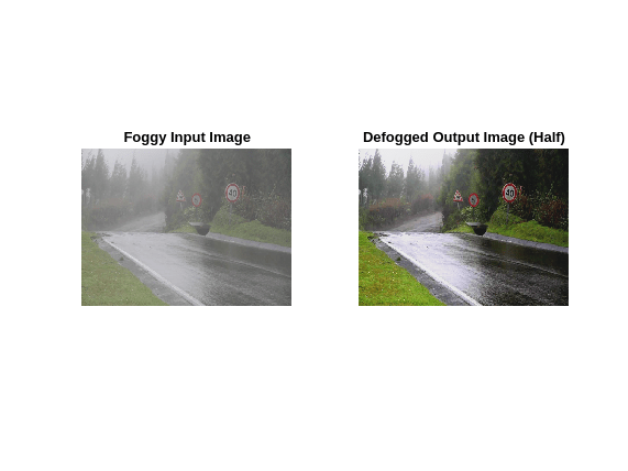
Run the Half-Precision MEX Function with Foggy Image
Run the generated fog_rectification_half_precision_mex with a foggy input image, and then plot the foggy and defogged images.
[outputImageHalf] = fog_rectification_half_precision_mex(inputImageHalf);

% plot images
p1  = subplot(1, 2, 1);
p2 = subplot(1, 2, 2);
imshow(inputImage, 'Parent', p1);
imshow(outputImageHalf, 'Parent', p2);
title(p1, 'Foggy Input Image');
title(p2, 'Defogged Output Image (Half)');

See Also
Functions
codegen|coder.gpu.kernel|coder.gpu.kernelfun|gpucoder.matrixMatrixKernel|coder.gpu.constantMemory|stencilfun|coder.checkGpuInstall