Generate GPU Code for a Multipath Propagation Function

Check GPU Environment

This example requires a compatible NVIDIA® GPU. To check that your GPU supports GPU code generation and execution, create a coder.gpuEnvConfig object, enable the BasicCodeexec property, and use the coder.checkGpuInstall function.

envCfg = coder.gpuEnvConfig;
envCfg.Quiet = true;
envCfg.BasicCodeexec = true;
coder.checkGpuInstall(envCfg);

Examine the Multipath Propagation Function

The multipathProp entry-point function takes information about the signal, transmitter, receivers, and scatterers, and returns a dechirped, frequency-domain representation of the received signal. The function:

type multipathProp.m

function receivedSig = multipathProp(sig, t, posTx, posRx, k, scattPos, scattCoeff)
% Given a linear frequency-modulated pulse, sig, in a multipath propagation
% scenario, return the dechirped, frequency-domain representation of
% the received signal.
% Inputs:
%   sig        - Transmitted chirp signal (1 x numSamples, complex single)
%   t          - Time vector for the pulse (1 x numSamples, single, seconds)
%   posTx      - Transmitter position (3 x 1, single, meters)
%   posRx      - Receiver position (3 x 1, single, meters)
%   k          - Chirp rate of the transmitted signal (scalar, single, Hz/s)
%   scattPos   - Initial scatterer positions (3 x numScatt, single, meters)
%   scattCoeff - Complex reflection coefficients (numScatt x 1, complex single)
% Output:
%   rec2DSig   - Range-pulse profile (nfft x 1, complex single).
%                Range profile for the pulse. Peaks
%                indicate scatterer locations.

coder.gpu.kernelfun;
c = single(physconst('lightspeed'));
numSamples = length(t);
nfft = 2^nextpow2(numSamples);
phaseConst = 1j*2*single(pi)*k;

% Compute propagation delays from transmitter to receiver for each path leg
incidentTd = sqrt(sum((scattPos - posTx).^2, 1)) / c; % TX to scatterer
reflectTd  = sqrt(sum((posRx - scattPos).^2, 1)) / c; % Scatterer to RX
totalTd    = incidentTd + reflectTd;

% Compute sum of scattered signals
receivedSignals = scattCoeff .* exp(phaseConst * ((t - totalTd.').^2 / 2));
superImposedSig = gpucoder.reduce(receivedSignals, @plus, dim=1);

% Because the input signal is LFM, dechirp to obtain signal whose component 
% frequencies correspond to propagation delays.
dechirpedSig = conj(superImposedSig) .* sig;

% Convert signal to frequency domain. Peaks correspond to component
% frequencies.
receivedSig = fft(dechirpedSig, nfft);
end

To generate code that uses the GPU, the function contains multiple code patterns that GPU Coder™ can parallelize. For example, the received signal is the sum of each reflected signal. To calculate the received signal by using the GPU, the function implements the sum by using the gpucoder.reduce function:

superImposedSig = gpucoder.reduce(receivedSignals, @plus, dim=1);

The generated code for gpucoder.reduce uses a kernel function to calculate the result. The generated code from multipathProp also maps this call to the fft function to the NVIDIA® cuFFT library:

receivedSig = fft(dechirpedSig, nfft);

The generated code uses the cuFFT library to compute the result on the GPU.

Test multipathProp Function

Test the multipathProp function. First, construct a linear chirp signal to send to transmit. Use the single data type.

c = single(physconst('lightspeed'));
fs = single(150e6);
bw = single(50e6);
maxRange = single(3000);
t = single(0:1/fs:maxRange/c);
k = single(bw/t(end));
sig = exp(1j*2*single(pi)*k*(t.^2/2));

Define the transmitter and receiver positions.

posTx = single([0;0;0]);
posRx = single([1000; 1000; 500]);

Create 10 scatterers at random positions. Assign each scatterer a random, complex scattering coefficient.

numScatt = 10;
rng("default");
scattPos = single(randi([100, 2000], 3, numScatt));
scattCoeff = single(randn(numScatt,1)) + 1j*single(randn(numScatt,1));

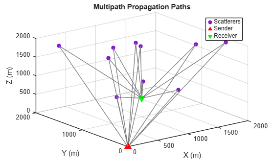
Use the plotScattererPositions helper function to plot the path from the transmitter to each scatterer and then to the receiver. The function creates a three-dimensional plot with lines from the receiver to each scatterer and from each scatterer to the transmitter.

plotScattererPositions(numScatt,posTx,scattPos,posRx);

Call the multipathProp function. Specify the signal and the transmitter, receiver, and scatterer positions as input arguments.

receivedSig = multipathProp(sig,t,posTx,posRx,k,scattPos,scattCoeff);

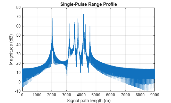
Use the visualizeRangeProfile helper function to plot the single-pulse range profile of the received signal by using the horizontal axis for the path length and the vertical axis for the signal magnitude in decibels. The plot shows 10 peaks whose locations correspond to the path length of each of the 10 scatterers. The heights of the peaks depend on the scattering coefficients.

visualizeRangeProfile(receivedSig,t,k);

Generate GPU Code

For GPU code generation, to generate code that executes faster because of the parallelism of the GPU, increase the number of scatterers to 500.

numScattLarge = 500;
rng("default");
scattPosLarge = single(randi([100, 2000], 3, numScattLarge));
scattCoeffLarge = single(randn(numScattLarge,1)) + 1j*single(randn(numScattLarge,1));

When you time generated GPU code, the execution time includes the time required to copy input data from the CPU to the GPU. To avoid including the time to copy inputs when you time multipathProp, load the scatterer positions and coefficients directly on the GPU by using gpuArray objects.

scattPosLarge_gpu = gpuArray(scattPosLarge);
scattCoeffLarge_gpu = gpuArray(scattCoeffLarge);
args = {sig,t,posTx,posRx,k,scattPosLarge_gpu,scattCoeffLarge_gpu};

Create a MEX code configuration by using the coder.gpuConfig function. To generate code, use the codegen command.

cfg = coder.gpuConfig("mex");
codegen multipathProp -args args -config cfg;

Code generation successful.

In the generated code file multipathProp.cu, the generated code calculates the superimposed signal by using the ReduceFirstDimBaseCaseKernel kernel function.

coder.example.extractLines(fullfile("codegen/mex/multipathProp/multipathProp.cu"),"ReduceFirstDimBaseCaseKernel<",");",true,true)

  ReduceFirstDimBaseCaseKernel<<<dim3(3U, 1U, 1U), dim3(128U, 1U, 1U)>>>(
      *b_gpu_inputArray, *gpu_tmp);

The code also uses the cuFFT library to calculate the output signal.

coder.example.extractLines(fullfile("codegen/mex/multipathProp/multipathProp.cu"),"mw::cufft",");",true,true)

  mw::cufftExecC2CInPlace(fftPlanHandle, (cufftComplex *)&receivedSig[0],
                          CUFFT_FORWARD);

Compare Output of Generated Code and the MATLAB Function

To compare the output of the GPU MEX function with the MATLAB function, compute the maximum relative error between the output of the GPU MEX function and MATLAB function.

cpuResult = multipathProp(sig, t, posTx, posRx, k, scattPosLarge, scattCoeffLarge);
gpuResult = multipathProp_mex(sig, t, posTx, posRx, k, scattPosLarge_gpu, scattCoeffLarge_gpu);

maxRelErr = max(abs(cpuResult - gpuResult), [], "all") / max(abs(cpuResult), [], "all");
disp("Maximum relative error (CPU vs GPU): " + maxRelErr)

Maximum relative error (CPU vs GPU): 1.1774e-07

The maximum relative error is on the order of ${10}^{-7}$, which is acceptable for single type inputs.

Compare the Execution Time of Generated Code and MATLAB

To compare the execution time of the generated code and MATLAB, use the timeit and gputimeit functions to time the MATLAB function and the CUDA® MEX function, respectively.

cpu_time = timeit(@() multipathProp(sig, t, posTx, posRx, k, scattPosLarge, scattCoeffLarge));
gpu_time = gputimeit(@() multipathProp_mex(sig, t, posTx, posRx, k, scattPosLarge_gpu, scattCoeffLarge_gpu));
gpu_speedup = cpu_time/gpu_time

gpu_speedup = 
561.6995

This output shows the speedup on a Windows 11 machine with a 13th Gen Intel® Core™ i9-13900K CPU and an NVIDIA GeForce RTX 3080 Ti GPU. The generated GPU code is more than 700 times faster than MATLAB simulation.

Helper Functions

The plotScattererPositions function generates a three-dimensional plot of the transmitter, receiver, and scatterer positions. The plot traces the paths from the transmitter to each scatterer to the receiver.

function plotScattererPositions(numScatt,posTx,scattPos,posRx)
figure
hold on
for jj = 1:numScatt
    plot3([posTx(1) scattPos(1,jj) posRx(1)], ...
        [posTx(2) scattPos(2,jj) posRx(2)], ...
        [posTx(3) scattPos(3,jj) posRx(3)], "-", Color=[0.5 0.5 0.5 0.5])
end
h1 = scatter3(scattPos(1,:), scattPos(2,:), scattPos(3,:), 40, "filled");
h2 = scatter3(posTx(1), posTx(2), posTx(3), 100, "r", "filled", "^");
h3 = scatter3(posRx(1), posRx(2), posRx(3), 100, "g", "filled", "v");
hold off
legend([h1 h2 h3],["Scatterers" "Sender" "Receiver"])
xlabel("X (m)")
ylabel("Y (m)")
zlabel("Z (m)")
title("Multipath Propagation Paths")
view(3)
grid on
end

The visualizeRangeProfile function plots the magnitude of the received signal, in decibels, over its path length, in meters.

function visualizeRangeProfile(receivedSig, t, k)
% Plot the single-pulse range profile in dB vs. path length.
%
% Inputs:
%   receivedSig - Output of multipathProp (nfft x 1, complex single)
%   t        - Time vector used for the pulse (1 x numSamples, single, seconds)
%   k        - Chirp rate (scalar, single, Hz/s)

c = single(physconst('lightspeed'));
fs = single(1/(t(2) - t(1)));
nfft = single(length(receivedSig));

beatFreq = single(0:fs/nfft:((nfft)-1)*fs/nfft); % compute frequency value for each bin
pathDist = c*beatFreq/k; % path length

figure;
plot(pathDist, mag2db(abs(receivedSig)));
xlabel("Signal path length (m)");
ylabel("Magnitude (dB)");
title("Single-Pulse Range Profile");
grid on;
end