Compressor (2P)

Two-phase fluid compressor in a thermodynamic cycle

Since R2022a

Libraries:
Simscape / Fluids / Two-Phase Fluid / Fluid Machines

Description

The Compressor (2P) block represents a dynamic compressor, such as a centrifugal or axial compressor, in a two-phase fluid network. You can use the Parameterization parameter to parameterize the block analytically based on the design point or by using a tabulated compressor map. A positive rotation of port R relative to port C causes fluid to flow from port A to port B. Port R and port C are mechanical rotational conserving ports associated with the compressor shaft and casing, respectively.

The surge margin is the ratio between the surge pressure ratio at a given mass flow rate and the operating point pressure ratio minus 1. When you set Parameterization to Tabulated, the block outputs the surge margin at port SM.

The design point is the design operational pressure ratio across and mass flow rate through the compressor during simulation. The compressor operating point and the point of maximum efficiency do not need to coincide.

The Compressor (2P) block assumes that superheated fluid enters the inlet. You can use the Report when fluid is not fully vapor parameter to choose what the block does when the fluid does not meet superheated conditions.

Compressor Map

The compressor map plots the isentropic efficiency of the compressor and the lines of constant corrected shaft speed between the two extremes of choked flow and surge flow. To visualize the block map, right-click the block and select Fluids > Plot Compressor Map. Each time you modify the block settings, click Reload Data on the figure window.

Compressor map

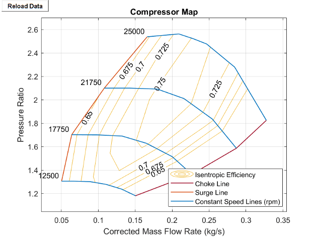
Each corrected speed line shows how the pressure ratio varies with the corrected mass flow rate when the shaft spins at the corresponding corrected speed. The variable β indicates the relative position along the corrected speed lines between the two extremes. Choked flow corresponds to β = 0 and surge flow corresponds to β = 1. The map also plots contours of isentropic efficiency as a function of pressure ratio and corrected mass flow rate, which provides a relative indication of how much power the compressor needs to operate at various combinations of pressure ratio and corrected mass flow rate.

Corrected Mass Flow Rate

Due to the large changes in pressure and temperature inside a compressor, the compressor map plots performance in terms of the corrected mass flow rate. The map adjusts the corrected mass flow rate from the inlet mass flow rate by using the reference pressure and reference temperature,

${\dot{m}}_{c o r r} = {\dot{m}}_{A} (\sqrt{\frac{T_{A}}{T_{r e f}}} / \frac{p_{A}}{p_{r e f}}),$

where:

ṁ_A is the mass flow rate at port A.
T_A is the temperature at port A.
T_ref is the value of the Reference temperature for corrected flow parameter. When you set Parameterization to Analytical, this is the inlet temperature at the design operating condition.
$\dot{m}$ _corr is the corrected mass flow rate. When you set Parameterization to Analytical, the block uses the Corrected mass flow rate at design point parameter. When you set Parameterization to Tabulated, the block uses the Corrected mass flow rate table, mdot(N,beta) parameter.
p_A is the pressure at port A.
p_ref is the Reference pressure for corrected flow parameter. When using the analytical parameterization, this is the inlet pressure at the design operating condition.

The block derives T_A from the specific internal energy, u_A, and specific pressure, p_A.

Corrected Speed

The block also adjusts the shaft speed, ω, according to the reference temperature, such that the corrected shaft speed is

$ω_{c o r r} = \frac{ω}{\sqrt{\frac{T_{A}}{T_{r e f}}}} .$

Shaft Torque

The block calculates the shaft torque, τ, as

$τ = \frac{{\dot{m}}_{A} Δ h_{t o t a l}}{η_{m} ω},$

where:

Δh_total is the change in specific total enthalpy.
η_m is the compressor Mechanical efficiency.
ω is the relative shaft angular velocity, ω_R - ω_C.

The block relates the efficiency in the compressor map as

$Δ h_{t o t a l} = \frac{Δ h_{i s e n}}{η_{i s e n}},$

where:

Δh_isen is the isentropic change in specific total enthalpy.
η_isen is the isentropic efficiency.

A threshold region when flow approaches zero ensures that the compressor generates no torque when the flow rate is near zero or reversed.

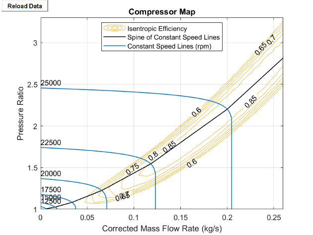
Analytical Parameterization

You can generate the compressor map analytically by setting Parameterization to Analytical. The block fits a model of the compressor map based on [1] to the specified values for the Corrected speed at design point, Pressure ratio at design point, and Corrected mass flow rate at design point parameters. This method does not use β lines and the block does not report a surge margin.

Pressure Ratio

The block finds the pressure ratio at a given shaft speed and mass flow rate as

$π = 1 + (π_{D} - 1) [{\tilde{N}}^{a b} + 2 \tilde{N} k \ln (1 - \frac{\tilde{m} - {\tilde{N}}^{b}}{k})],$

where:

π_D is the Pressure ratio at design point parameter.
$\tilde{N}$ is the normalized corrected shaft speed,

$\frac{N}{N_{D}},$
where N_D is the Corrected speed at design point parameter.
$\tilde{m}$ is the normalized corrected mass flow rate,

$\frac{{\dot{m}}_{c o r r}}{{\dot{m}}_{D}},$
where $\dot{m}$ _D is the Corrected mass flow rate at design point parameter.
a is the Spine shape, a parameter.
b is the Speed line spread, b parameter.
k is the Speed line roundness, k parameter.

The spine refers to the black line where the isentropic efficiency contours start to bend. The map speed lines are the shaft constant-speed lines that intersect the spine perpendicularly.

Compressor analytical map

Isentropic Efficiency Parameterization

When you set Efficiency specification to Analytical, the block models variable compressor efficiency as

$η = η_{0} (1 - C {| \frac{\tilde{p}}{{\tilde{m}}^{a + Δ a - 1}} - \tilde{m} |}^{c} - D {| \frac{\tilde{m}}{{\tilde{m}}_{0}} - 1 |}^{d}),$

where:

η₀ is the value of the Maximum isentropic efficiency parameter.
C is the value of the Efficiency contour gradient orthogonal to spine, C parameter.
D is the value of the Efficiency contour gradient along spine, D parameter.
c is the value of the Efficiency peak flatness orthogonal to spine, c parameter.
d is the value of the Efficiency peak flatness along spine, d parameter.
$\tilde{p}$ is the normalized corrected pressure ratio,

$\frac{π - 1}{π_{D} - 1},$
where π_D is the Corrected pressure ratio at design point parameter.
$\tilde{m}$ ₀ is the normalized corrected mass flow rate at which the compressor reaches the value of the Maximum isentropic efficiency parameter.

You can adjust the efficiency variables for different performance characteristics. Alternatively, you can choose a constant efficiency value by using the Constant isentropic efficiency parameter.

Tabulated Data Parameterization

When you set Parameterization to Tabulated, the isentropic efficiency, pressure ratio, and corrected mass flow rate of the compressor are functions of the corrected speed, N, and the map index, β. The block uses linear interpolation between data points for the efficiency, pressure ratio, and corrected mass flow rate.

If β exceeds 1, compressor surge occurs and the block assumes the pressure ratio remains at β = 1, while the mass flow rate continues to change. If the simulation conditions fall below β = 0, the block models the effects of choked flow, where the mass flow rate remains at its value at β = 0 while the pressure ratio continues to change. To constrain the compressor performance in the map boundaries, the block extrapolates isentropic efficiency to the nearest point.

You can choose to be notified when the operating point pressure ratio exceeds the surge pressure ratio. Set Report when surge margin is negative to Warning to receive a warning or to Error to stop the simulation when this occurs.

Continuity Equations

The block conserves mass such that

${\dot{m}}_{A} + {\dot{m}}_{B} = 0,$

where $\dot{m}$ _B is the mass flow rate at port B.

The block computes the energy balance equation as

$Φ_{A} + Φ_{B} + P_{f l u i d} = 0,$

where:

Φ_A is the energy flow rate at port A.
Φ_B is the energy flow rate at port B.
P_fluid is the hydraulic power delivered to the fluid,which the block determines from the change in specific enthalpy $P_{f l u i d} = {\dot{m}}_{A} Δ h_{t o t a l} .$

Assumptions and Limitations

The block assumes that superheated fluid enters at A.
The block only defines compressor map flow from port A to port B. Reverse flow results may not be accurate.
The block only represents dynamic compressors.

Ports

Output

expand all

SM — Surge margin
physical signal

Physical signal output port associated with the surge margin at a given mass flow rate. The block calculates the surge margin as

$S M ({\dot{m}}_{c o r r}) = \frac{p_{r, s u r g e} ({\dot{m}}_{c o r r})}{p_{r} ({\dot{m}}_{c o r r})} - 1.$

Dependencies

To enable this port, set Parameterization to Tabulated.

Conserving

expand all

A — Compressor inlet
two-phase fluid

Two-phase fluid conserving port associated with the compressor inlet.

B — Compressor outlet
two-phase fluid

Two-phase fluid conserving port associated with the compressor outlet.

C — Compressor casing
mechanical rotational

Mechanical rotational conserving port associated with the compressor case.

R — Compressor shaft
mechanical rotational

Mechanical rotational conserving port associated with the compressor shaft.

Parameters

expand all

Compressor Map

Parameterization — Compressor performance parameterization
`Analytical` (default) | `Tabulated`

Compressor performance parameterization. Choose the analytical or tabulated parameterization:

Analytical: A pressure ratio–corrected mass flow rate curve defines the peak compressor performance. You can choose to model isentropic efficiency as a constant or analytically.
Tabulated: A user-supplied compressor map defines the compressor performance. The block determines the compressor operating points by using linear interpolation between the corrected mass flow rate, pressure ratio, and isentropic efficiency tables at given points in the user-provided corrected shaft speed and β vectors. The default map comes from data reported in [3].

Corrected speed at design point — Operational corrected shaft speed
`25000` `rpm` (default) | positive scalar

Shaft speed at the intended compressor pressure ratio and corrected mass flow rate, corrected for temperature.

Dependencies

To enable this parameter, set Parameterization to Analytical.

Pressure ratio at design point — Operational outlet-to-inlet pressure ratio
`2.2` (default) | positive scalar

Outlet-to-inlet pressure ratio at the intended compressor corrected mass flow rate.

Dependencies

To enable this parameter, set Parameterization to Analytical.

Corrected mass flow rate at design point — Operational corrected mass flow rate
`0.20` `kg/s` (default) | positive scalar

Mass flow rate at the intended compressor pressure ratio, corrected for temperature and pressure.

Dependencies

To enable this parameter, set Parameterization to Analytical.

Efficiency specification — Isentropic efficiency option
`Constant` (default) | `Analytical`

Isentropic efficiency model type. Choose a constant or analytical model. Use Analytical to specify variable values.

Dependencies

To enable this parameter, set Parameterization to Analytical.

Maximum isentropic efficiency — Maximum compressor efficiency
`0.887` (default) | positive scalar in the range (0,1]

Maximum compressor isentropic efficiency. Isentropic efficiency is the ratio of isentropic change to actual change.

Dependencies

To enable this parameter, set Parameterization to Analytical and Efficiency specification to Analytical.

Minimum isentropic efficiency — Minimum compressor efficiency
`0.5` (default) | positive scalar in the range (0,1]

Minimum compressor isentropic efficiency. Isentropic efficiency is the ratio of isentropic change to actual change.

Dependencies

To enable this parameter, set Parameterization to Analytical and Efficiency specification to Analytical.

Corrected mass flow rate at maximum efficiency point — Corrected mass flow rate at compressor maximum efficiency
`0.19` `kg/s` (default) | positive scalar

Mass flow rate at maximum efficiency, corrected for temperature and pressure. The point of maximum efficiency does not necessarily coincide with the compressor design point.

Dependencies

To enable this parameter, set Parameterization to Analytical and Efficiency specification to Analytical.

Pressure ratio at maximum efficiency point — Pressure ratio at compressor maximum efficiency
`2.1` (default) | positive scalar

Pressure ratio at maximum efficiency. The point of maximum efficiency does not necessarily coincide with the compressor design point.

Dependencies

To enable this parameter, set Parameterization to Analytical and Efficiency specification to Analytical.

Constant isentropic efficiency — Constant isentropic efficiency value
`0.8` (default) | positive scalar

Value of the constant isentropic efficiency.

Dependencies

To enable this parameter, set Parameterization to Analytical and Efficiency specification to Constant.

Corrected speed index vector, N — Vector of corrected shaft speeds
`[12500, 17750, 21750, 25000]` rpm (default) | vector

Vector of corrected shaft speeds.

Dependencies

To enable this parameter, set Parameterization to Tabulated.

Beta index vector, beta — Vector of corrected speed line intervals
`0 : 1 / 5 : 1` (default) | vector of elements in the range [0,1]

Vector of relative positions along the corrected speed lines. Choked flow occurs when β = 0 and surge flow occurs at β = 1. β lines are perpendicular to the compressor shaft constant speed lines, N.

Dependencies

To enable this parameter, set Parameterization to Tabulated.

Pressure ratio table, pr(N, beta) — Compressor map pressure ratio data
M-by-N matrix (default)

M-by-N matrix of compressor outlet-to-inlet pressure ratios at the specified corrected shaft speed and β value. The block employs linear interpolation between table elements. M and N are the sizes of the corresponding vectors:

M is the number of vector elements in the Corrected speed index vector, N parameter.
N is the number of vector elements in the Beta index vector, beta parameter.

The default value is:

[1.1814, 1.2385, 1.2792, 1.3017, 1.3057, 1.3057; 1.3648, 1.5157, 1.6298, 1.691, 1.7011, 1.7032; 1.587, 1.8357, 2.011, 2.0925, 2.1006, 2.1006; 1.8255, 2.28, 2.4777, 2.5225, 2.5633, 2.5389]

Dependencies

To enable this parameter, set Parameterization to Tabulated.

Corrected mass flow rate table, mdot(N,beta) — Compressor map corrected mass flow rate data
M-by-N matrix (default)

M-by-N matrix of corrected mass flow rates at the specified corrected shaft speed and β value. The block employs linear interpolation between table elements. M and N are the sizes of the corresponding vectors:

M is the number of vector elements in the Corrected speed index vector, N parameter.
N is the number of vector elements in the Beta index vector, beta parameter.

The default value is:

[.1503, .1313, .11, .0887, .0668, .0502; .2265, .1999, .1649, .1322, .0992, .0639; .2869, .2545, .216, .1798, .1424, .108; .3275, .2846, .2466, .2285, .209, .1661] kg/s

Dependencies

To enable this parameter, set Parameterization to Tabulated.

Isentropic efficiency table, eta(N,beta) — Compressor map isentropic efficiency data
M-by-N matrix (default)

M-by-N matrix of compressor isentropic efficiencies at the specified corrected shaft speed and β value. The block employs linear interpolation between table elements. M and N are the sizes of the corresponding vectors:

M is the number of vector elements in the Corrected speed index vector, N parameter.
N is the number of vector elements in the Beta index vector, beta parameter.

The default value is:

[.56, .66, .71, .695, .659, .635; .558, .682, .755, .743, .697, .638; .57, .705, .765, .752, .712, .652; .552, .718, .755, .752, .736, .67]

Dependencies

To enable this parameter, set Parameterization to Tabulated.

Report when surge margin is negative — Negative surge margin notification
`None` (default) | `Warning` | `Error`

Whether the block does nothing, generates a warning, or generates an error when it detects a negative surge margin.

Dependencies

To enable this parameter, set Parameterization to Tabulated.

Map Coefficients

To enable the Map Coefficients parameters, set Parameterization to Analytical.

Spine shape, a — Spine shape exponent
`1.5` (default) | positive scalar

Exponent in the analytical parameterization of the compressor map that characterizes the spine shape.

Dependencies

To enable this parameter, set Parameterization to Analytical.

Speed line spread, b — Constant speed line spacing exponent
`5` (default) | positive scalar

Exponent in the analytical parameterization of the compressor map that characterizes the constant speed line spacing.

Dependencies

To enable this parameter, set Parameterization to Analytical.

Speed line roundness, k — Constant speed line shape coefficient
`0.03` (default) | positive scalar

Coefficient in the analytical parameterization of the compressor map that characterizes the constant speed line shape.

Dependencies

To enable this parameter, set Parameterization to Analytical.

Efficiency peak flatness orthogonal to spine, c — Flatness orthogonal to spine exponent
`3` (default) | positive scalar

Exponent associated with the compressor map peak flatness orthogonal to the spine.

Dependencies

To enable this parameter, set Parameterization to Analytical and Efficiency specification to Analytical.

Efficiency peak flatness along spine, d — Along spine flatness exponent
`4` (default) | positive scalar

Exponent associated with the efficiency map peak flatness along the spine.

Dependencies

To enable this parameter, set Parameterization to Analytical and Efficiency specification to Analytical.

Efficiency contour gradient orthogonal to spine, C — Orthogonal gradient coefficient
`15` (default) | positive scalar

Coefficient associated with the efficiency contour gradient orthogonal to the spine.

Dependencies

To enable this parameter, set Parameterization to Analytical and Efficiency specification to Analytical.

Efficiency contour gradient along spine, D — Along spine gradient coefficient
`1` (default) | positive scalar

Coefficient associated with the efficiency contour gradient along the spine.

Dependencies

To enable this parameter, set Parameterization to Analytical and Efficiency specification to Analytical.

Reference data

Reference pressure for corrected flow — Correcting pressure
`0.101325` `MPa` (default) | positive scalar

Reference inlet pressure for the compressor map. When you set Parameterization to Tabulated, the data supplier specifies this value with respect to the tabulated compressor data. When you set Parameterization to Analytical, this value is the inlet pressure at the design operating condition.

Reference temperature for corrected flow — Correcting temperature
`373.15` `K` (default) | positive scalar

Reference inlet temperature for the compressor map. When you set Parameterization to Tabulated, the data supplier specifies this value with respect to the tabulated compressor data. When you set Parameterization to Analytical, this value is the inlet temperature at the design operating condition.

Mechanical efficiency — Efficiency of conversion to torque
`0.9` (default) | positive scalar in the range [0,1]

Ratio of the power delivered to the fluid flow to the power driving the mechanical shaft.

Inlet area at port A — Compressor inlet area
`0.01` `m^2` (default) | positive scalar

Compressor inlet cross-sectional area.

Outlet area at port B — Compressor outlet area
`0.01` `m^2` (default) | positive scalar

Compressor outlet cross-sectional area.

Report when fluid at inlet is not fully vapor — Fluid not fully vapor notification
`None` (default) | `Warning` | `Error`

Whether the block does nothing, generates a warning, or generates an error when it detects fluid that is not fully vapor.

References

[1] Greitzer, E. M. et al. “N+3 Aircraft Concept Designs and Trade Studies. Volume 2: Appendices – Design Methodologies for Aerodynamics, Structures, Weight, and Thermodynamic Cycles.” NASA Technical Report, 2010.

[2] Kurzke, Joachim. "How to Get Component Maps for Aircraft Gas Turbine Performance Calculations." Volume 5: Manufacturing Materials and Metallurgy; Ceramics; Structures and Dynamics; Controls, Diagnostics and Instrumentation; Education; General, American Society of Mechanical Engineers, 1996, p. V005T16A001.

[3] Plencner, Robert M. “Plotting component maps in the Navy/NASA Engine Program (NNEP): A method and its usage.” NASA Technical Memorandum, 1989.

Extended Capabilities

C/C++ Code Generation
Generate C and C++ code using Simulink® Coder™.

Version History

Introduced in R2022a

Compressor (2P)

Description

Compressor Map

Shaft Torque

Analytical Parameterization

Tabulated Data Parameterization

Continuity Equations

Assumptions and Limitations

Ports

Output

SM — Surge margin physical signal

Dependencies

Conserving

A — Compressor inlet two-phase fluid

B — Compressor outlet two-phase fluid

C — Compressor casing mechanical rotational

R — Compressor shaft mechanical rotational

Parameters

Compressor Map

Parameterization — Compressor performance parameterization Analytical (default) | Tabulated

Corrected speed at design point — Operational corrected shaft speed 25000 rpm (default) | positive scalar

Dependencies

Pressure ratio at design point — Operational outlet-to-inlet pressure ratio 2.2 (default) | positive scalar

Dependencies

Corrected mass flow rate at design point — Operational corrected mass flow rate 0.20 kg/s (default) | positive scalar

Dependencies

Efficiency specification — Isentropic efficiency option Constant (default) | Analytical

Dependencies

Maximum isentropic efficiency — Maximum compressor efficiency 0.887 (default) | positive scalar in the range (0,1]

Dependencies

Minimum isentropic efficiency — Minimum compressor efficiency 0.5 (default) | positive scalar in the range (0,1]

Dependencies

Corrected mass flow rate at maximum efficiency point — Corrected mass flow rate at compressor maximum efficiency 0.19 kg/s (default) | positive scalar

Dependencies

Pressure ratio at maximum efficiency point — Pressure ratio at compressor maximum efficiency 2.1 (default) | positive scalar

Dependencies

Constant isentropic efficiency — Constant isentropic efficiency value 0.8 (default) | positive scalar

Dependencies

Corrected speed index vector, N — Vector of corrected shaft speeds [12500, 17750, 21750, 25000] rpm (default) | vector

Dependencies

Beta index vector, beta — Vector of corrected speed line intervals 0 : 1 / 5 : 1 (default) | vector of elements in the range [0,1]

Dependencies

Pressure ratio table, pr(N, beta) — Compressor map pressure ratio data M-by-N matrix (default)

Dependencies

Corrected mass flow rate table, mdot(N,beta) — Compressor map corrected mass flow rate data M-by-N matrix (default)

Dependencies

Isentropic efficiency table, eta(N,beta) — Compressor map isentropic efficiency data M-by-N matrix (default)

Dependencies

Report when surge margin is negative — Negative surge margin notification None (default) | Warning | Error

Dependencies

Map Coefficients

Spine shape, a — Spine shape exponent 1.5 (default) | positive scalar

Dependencies

Speed line spread, b — Constant speed line spacing exponent 5 (default) | positive scalar

Dependencies

Speed line roundness, k — Constant speed line shape coefficient 0.03 (default) | positive scalar

Dependencies

Efficiency peak flatness orthogonal to spine, c — Flatness orthogonal to spine exponent 3 (default) | positive scalar

Dependencies

Efficiency peak flatness along spine, d — Along spine flatness exponent 4 (default) | positive scalar

Dependencies

Efficiency contour gradient orthogonal to spine, C — Orthogonal gradient coefficient 15 (default) | positive scalar

Dependencies

Efficiency contour gradient along spine, D — Along spine gradient coefficient 1 (default) | positive scalar

Dependencies

Reference data

Reference pressure for corrected flow — Correcting pressure 0.101325 MPa (default) | positive scalar

Reference temperature for corrected flow — Correcting temperature 373.15 K (default) | positive scalar

Mechanical efficiency — Efficiency of conversion to torque 0.9 (default) | positive scalar in the range [0,1]

Inlet area at port A — Compressor inlet area 0.01 m^2 (default) | positive scalar

Outlet area at port B — Compressor outlet area 0.01 m^2 (default) | positive scalar

Report when fluid at inlet is not fully vapor — Fluid not fully vapor notification None (default) | Warning | Error

References

Extended Capabilities

C/C++ Code Generation Generate C and C++ code using Simulink® Coder™.

Version History

See Also

WeChat

SM — Surge margin
physical signal

A — Compressor inlet
two-phase fluid

B — Compressor outlet
two-phase fluid

C — Compressor casing
mechanical rotational

R — Compressor shaft
mechanical rotational

Parameterization — Compressor performance parameterization
`Analytical` (default) | `Tabulated`

Corrected speed at design point — Operational corrected shaft speed
`25000` `rpm` (default) | positive scalar

Pressure ratio at design point — Operational outlet-to-inlet pressure ratio
`2.2` (default) | positive scalar

Corrected mass flow rate at design point — Operational corrected mass flow rate
`0.20` `kg/s` (default) | positive scalar

Efficiency specification — Isentropic efficiency option
`Constant` (default) | `Analytical`

Maximum isentropic efficiency — Maximum compressor efficiency
`0.887` (default) | positive scalar in the range (0,1]

Minimum isentropic efficiency — Minimum compressor efficiency
`0.5` (default) | positive scalar in the range (0,1]

Corrected mass flow rate at maximum efficiency point — Corrected mass flow rate at compressor maximum efficiency
`0.19` `kg/s` (default) | positive scalar

Pressure ratio at maximum efficiency point — Pressure ratio at compressor maximum efficiency
`2.1` (default) | positive scalar

Constant isentropic efficiency — Constant isentropic efficiency value
`0.8` (default) | positive scalar

Corrected speed index vector, N — Vector of corrected shaft speeds
`[12500, 17750, 21750, 25000]` rpm (default) | vector

Beta index vector, beta — Vector of corrected speed line intervals
`0 : 1 / 5 : 1` (default) | vector of elements in the range [0,1]

Pressure ratio table, pr(N, beta) — Compressor map pressure ratio data
M-by-N matrix (default)

Corrected mass flow rate table, mdot(N,beta) — Compressor map corrected mass flow rate data
M-by-N matrix (default)

Isentropic efficiency table, eta(N,beta) — Compressor map isentropic efficiency data
M-by-N matrix (default)

Report when surge margin is negative — Negative surge margin notification
`None` (default) | `Warning` | `Error`

Spine shape, a — Spine shape exponent
`1.5` (default) | positive scalar

Speed line spread, b — Constant speed line spacing exponent
`5` (default) | positive scalar

Speed line roundness, k — Constant speed line shape coefficient
`0.03` (default) | positive scalar

Efficiency peak flatness orthogonal to spine, c — Flatness orthogonal to spine exponent
`3` (default) | positive scalar

Efficiency peak flatness along spine, d — Along spine flatness exponent
`4` (default) | positive scalar

Efficiency contour gradient orthogonal to spine, C — Orthogonal gradient coefficient
`15` (default) | positive scalar

Efficiency contour gradient along spine, D — Along spine gradient coefficient
`1` (default) | positive scalar

Reference pressure for corrected flow — Correcting pressure
`0.101325` `MPa` (default) | positive scalar

Reference temperature for corrected flow — Correcting temperature
`373.15` `K` (default) | positive scalar

Mechanical efficiency — Efficiency of conversion to torque
`0.9` (default) | positive scalar in the range [0,1]

Inlet area at port A — Compressor inlet area
`0.01` `m^2` (default) | positive scalar

Outlet area at port B — Compressor outlet area
`0.01` `m^2` (default) | positive scalar

Report when fluid at inlet is not fully vapor — Fluid not fully vapor notification
`None` (default) | `Warning` | `Error`

C/C++ Code Generation
Generate C and C++ code using Simulink® Coder™.