Pressure Loss and Mass Flow Rate in a Thermal Liquid Pipe
This example shows how changes in pipe and fluid attributes, such as friction and elevation change, impact the pressure loss through a pipe and how enabling dynamic compressibility impacts the mass flow rate. These effects are especially important in long, narrow pipes because they ensure the flow pressure is strong enough to overcome the pressure loss. This example uses the Simscape™ Fluids™ Pipe (TL) block.
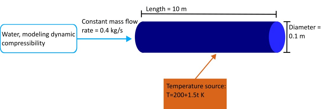
For this example, suppose you have a pipe that is 10 meters long with a circular cross-section and a 0.1 meter diameter. The mass flow rate into the pipe is constant at 0.4 kg/s and comes from a reservoir with water at 293.15 K and atmospheric pressure. Initially, the pipe does not include the effects of fluid dynamic compressibility.

Create MATLAB® parameters to represent the mass flow rate, pipe length, and pipe diameter.
mdot         = 0.4;  %   [kg/s] Mass flow rate
length       = 10;   %   [m]   Pipe length
D            = 0.1;  %   [m]   Pipe diameter
Pressure Loss Due to Change in Elevation
Consider the same pipe with a change in elevation of 3 meters. Ignoring the effects of friction, calculate the pressure loss due to elevation over the pipe analytically and the use a Simscape model to verify your results.
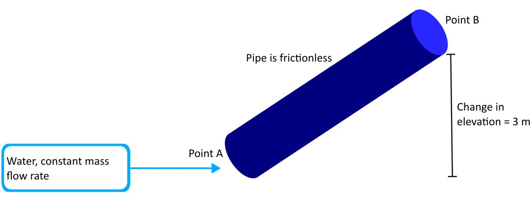
The pressure difference over the pipe is the sum of the pressure loss due to friction at the pipe wall and pressure loss due to a change in elevation,
![]()
where ![]() is the pressure drop due to a change in elevation across the pipe and
is the pressure drop due to a change in elevation across the pipe and ![]() is the pressure drop due to friction at the pipe wall. Because you ignore the effects of friction, set the
is the pressure drop due to friction at the pipe wall. Because you ignore the effects of friction, set the ![]() term to zero and use Bernoulli's Principle to determine an expression for
term to zero and use Bernoulli's Principle to determine an expression for ![]() .
.
Bernoulli's Principle is an important concept in fluid dynamics that relates the speed, pressure, and height of a fluid at different locations. You can use Bernoulli's Principle to calculate the properties of a fluid that flows between points A and B and ignores the effects of friction. Bernoulli's Principle states
![]()
where:
is the pressure at point A or point B.
ρ is the fluid density.
v is the fluid velocity at point A or point B.
g is acceleration due to gravity.
h is the fluid height at point A or point B.
When you model an incompressible fluid, mass is conserved and ![]() , where:
, where:
 is the mass flow rate at point A.
 is the mass flow rate at point B.
Mass flow rate is the product of the density, velocity, and cross-sectional area. Because , if you assume that fluid density and the pipe cross-sectional area are constant through the pipe, then and the velocity terms cancel off both sides of the Bernoulli's Principle equation. Grouping the remaining terms yields
![]()
where ![]() is the change in height from point A to point B.
is the change in height from point A to point B.
Use this analytical expression to calculate the expected pressure loss due to change in elevation. Adjust the value of ![]() to change the elevation change of the pipe.
to change the elevation change of the pipe.
delta_z  = 3;    %   [m]      Elevation gain
g        = 9.81; %   [m/s^2]  Gravity
rho      = 998;  %   [kg/m^3] Density of water at 293 K and 0.1325 MPa

deltaP_h = rho*g*delta_z % [Pa] Analytical pressure drop due to change in elevation
deltaP_h =
2.9371e+04
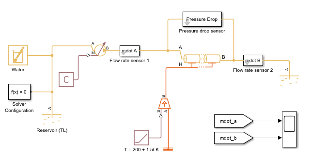
You can also use a Simscape model to confirm the analytical results. Open the PressureLossAndFlowRateInTLPipeInsulated model, which models constant flow through a pipe between two reservoirs. The model conditions match the conditions described above.
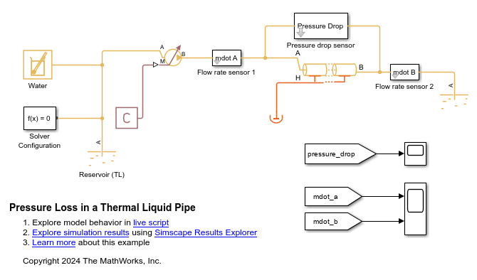
mdl ='PressureLossAndFlowRateInTLPipeInsulated';
open_system(mdl);
sim(mdl);
Plot the simulation output and examine the results.
t       = tout;          %  [sec]  Time
delta_P = pressure_drop; %  [Pa]  Pressure drop
plot(t, delta_P)
ylim([2.93e4, 2.94e4])
xlabel('Time (s)')
ylabel('Pressure Drop (Pa)')
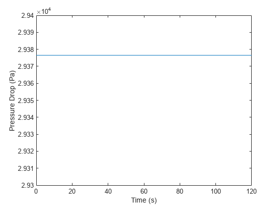
You cannot fully disable friction in the Pipe (TL) block, so the model results contain the pressure loss due to friction. However, this pressure loss is much smaller in magnitude than the pressure loss due to elevation gain. The model results show a constant pressure loss of about Pa, which agrees with the analytical results.
Pressure Loss Due to Friction
The magnitude of the pressure change due to friction, ![]() , is typically much smaller than the pressure change due to elevation change. However, if
, is typically much smaller than the pressure change due to elevation change. However, if ![]() is zero,
is zero, ![]() is the primary cause of pressure loss in the pipe.
is the primary cause of pressure loss in the pipe.
Consider a pipe with an inner wall surface made of brass, which has a surface absolute roughness of m. Calculate the pressure loss due to friction over the pipe analytically and then use a Simscape model to verify your results.

The expression for the pressure loss due to friction depends on the Reynolds number of the fluid. The Reynolds number is a dimensionless value used in fluid dynamics to help predict fluid flow patterns. It represents the ratio of fluid momentum to fluid viscous forces. At low Reynolds numbers, fluids tend to be more laminar, but their behavior can become more turbulent as the Reynolds number increases. The Reynolds number is
![]()
where:
v is the velocity of the flow.
μ is the fluid dynamic viscosity.
D is the pipe diameter.
Use the expression for the mass flow rate, ![]() , to rewrite the expression as
, to rewrite the expression as
![]()
where A is the cross-sectional area of the pipe. Calculate the Reynolds number for the water in the pipe.
area = pi/4*D^2;  % [m^2]   Pipe cross-sectional area
mu   = 0.00102;   % [Pa*s]  Dynamic viscosity of water at 293 K and 0.101325 MPa

Re   = mdot*D/(area*mu)  % Reynolds number
Re =
4.9931e+03
A Reynolds number greater than 4000 is typically considered a turbulent flow, which means the flow is characterized by chaotic changes in pressure and velocity. The pressure loss due to friction in the turbulent regime is
![]()
where:
L is the pipe length.
f is the Darcy friction factor.
The Darcy friction factor is a dimensionless value that describes the friction resistance in a pipe [1]. Friction resistance is the effect of the interior surface of a pipe creating friction against the fluid flowing through it. This friction slows down the flow, which causes the pressure drop due to friction,
![]()
where ϵ is the measure of the internal surface absolute roughness.
epsilon = 1.52e-6;   %  [m]     Internal surface absolute roughness for commercial brass, lead, copper, or plastic pipe

f        = 1 / (-1.8 * log10(6.9/Re + (epsilon/3.7)^1.11))^2; %      Darcy friction factor
deltaP_f = f * length * mdot * abs(mdot) / (2*rho*D*area^2)   % [Pa] Pressure loss due to friction
deltaP_f =
4.9052
Use the PressureLossAndFlowRateInTLPipeInsulated model to confirm the value of the pressure loss due to friction.
mdl = 'PressureLossAndFlowRateInTLPipeInsulated';
delta_z = 0;               %  [m] Pipe elevation
open_system(mdl);
sim(mdl);
Plot the simulation output and examine the results.
t = tout;                   % [sec] Time
delta_P = pressure_drop;    % [Pa]  Pressure drop
plot(t, delta_P)
ylim([4.85, 4.95])
xlabel('Time (s)')
ylabel('Pressure Drop (Pa)')
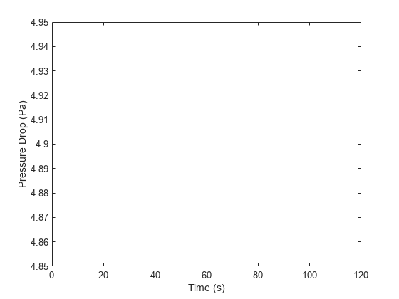
The model results show a constant pressure loss of about 4.907 Pa, which agrees with the analytical prediction of 4.905 Pa. The values differ because the density and viscosity vary slightly in the simulation.
Different pipe wall materials have different values for the interior surface absolute roughness. Calculate the pressure loss due to friction for multiple pipe materials to examine the impact material can have on pressure loss.
Material  = {'Brass, lead, copper, or plastic'; 'Steel or wrought iron';'New cast iron';'Rusty cast iron'};
Roughness = [1.52e-6; 4.6e-5; 2.59e-4; 1.5e-3]; % [m] Internal surface absolute roughness

f         = 1 ./ (-1.8 * log10(6.9/Re + (Roughness./3.7).^1.11)).^2;  %      Darcy friction factor
Pressure_Loss  = f * length * mdot * abs(mdot) ./ (2*rho*D*area^2);   % [Pa] Pressure loss due to friction
T = table (Material, Roughness, Pressure_Loss)T=4×3 table
Material Roughness Pressure_Loss
___________________________________ _________ _____________
{'Brass, lead, copper, or plastic'} 1.52e-06 4.9052
{'Steel or wrought iron' } 4.6e-05 4.909
{'New cast iron' } 0.000259 4.9313
{'Rusty cast iron' } 0.0015 5.0844
This table shows how pressure loss due to friction depends on the pipe material or condition. These differences have small magnitudes but they cause comparatively large pressure drops in highly sensitive systems.
Mass Balance and Fluid Compressibility
Use mass balance equations and a Simscape model to investigate the effects of enabling fluid dynamic compressibility and introducing a heat source on the pipe mass flow rate.
When you clear the Fluid dynamic compressibility parameter in a pipe block, such as a Pipe (TL) block, there is no accumulation of mass in the pipe and the mass inflow equals mass outflow,
![]() ,
,
where:
is the mass flow rate into port A.
is the mass flow rate into port B.
If you simulate the model, you can verify this behavior. There is no difference between the mass flow rates entering and leaving the pipe. Because the flow rates are equal and opposite, the plot shows the negative of ![]() . Open and simulate the
. Open and simulate the PressureLossAndFlowRateInTLPipeInsulated model.
mdl = 'PressureLossAndFlowRateInTLPipeInsulated';
open_system(mdl);
sim(mdl);
Get the simulation results and plot them.
t = tout;                           % [sec]  Time
mdot_a_incompressible = mdot_a;     % [kg/s] Mass flow rate into port A
mdot_b_incompressible = mdot_b;     % [kg/s] Mass flow rate into port B
plot(t,mdot_a_incompressible,t,-mdot_b_incompressible,'--')
xlabel('Time (s)')
ylabel('Mass flow rate (kg/s)')
legend('mdot_a','-mdot_b')
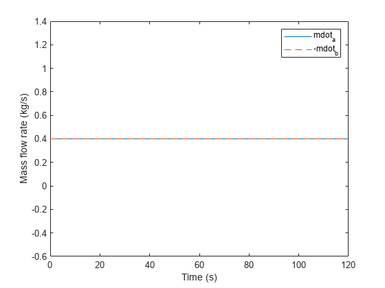
The mass flow rate at ports A and B are equal in magnitude and opposite in sign.
This behavior can change if you enable fluid dynamic compressibility. Because compressible fluid can accumulate in the pipe, the mass balance equation has additional terms,
![]()
where:
V is the pipe fluid volume.
ρ is the density.
p is the pressure.
T is the temperature.
β is the isothermal bulk modulus.
α is the isobaric thermal expansion coefficient.
Because the pipe is perfectly insulated and the pressure loss due to friction is insignificant, ![]() and are both negligible. In this scenario, because the right side of the mass balance equation is still approximately zero, the pipe behaves the same as in the incompressible case and there is no change in the mass flow rate from port A to port B.
and are both negligible. In this scenario, because the right side of the mass balance equation is still approximately zero, the pipe behaves the same as in the incompressible case and there is no change in the mass flow rate from port A to port B.
Enable dynamic compressibility in the pipe block.
set_param('PressureLossAndFlowRateInTLPipeInsulated/Pipe (TL)','dynamic_compressibility','true')
When the pipe block models dynamic compressibility, you can also specify the value of the Initial liquid pressure parameter. To minimize the spike in the mass flow rate when the time is 0, initialize the pressure in the pipe to the average of the pressure in the two reservoirs, and account for pressure loss. Both reservoirs are at atmospheric pressure, or 0.101327 MPa. The pressure at the midpoint of the pipe is the atmospheric pressure plus half of the pressure loss over the pipe. Use the value of the pressure loss due to friction from the previous section to calculate the value for the Initial liquid pressure parameter, and set the parameter to this value.
p_atm = 0.101327;                 % [MPa] Atmospheric pressure
deltaP_f_MPa = deltaP_f*1e-6;     % [MPa] Pressure loss due to friction in MPa
p_I = p_atm + deltaP_f_MPa/2;     % [MPa] Initial pressure at the pipe midpoint

set_param('PressureLossAndFlowRateInTLPipeInsulated/Pipe (TL)','p0_vec','p_I')
Simulate the model, plot the output, and examine the results.
sim(mdl);

figure
t = tout;                       % [sec]  Time
mdot_a_compressible = mdot_a;   % [kg/s] Mass Flow rate into port A
mdot_b_compressible = mdot_b;   % [kg/s] Mass flow rate into port B
plot(t,mdot_a_compressible,t,-mdot_b_compressible,'--')
ylim([.39, .41])
xlabel('Time (s)')
ylabel('Mass flow rate (kg/s)')
legend('mdot_a','-mdot_b')

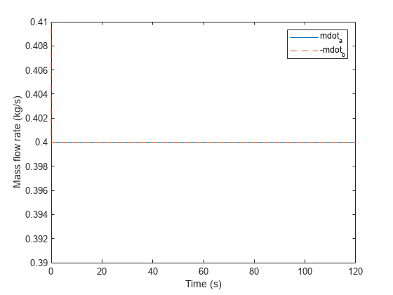
The mass flow rates at ports A and B are equal in magnitude and opposite in sign.
However, if you initiate heat transfer by including a heat source, is no longer negligible. Consider a model where the temperature of the heat source connected to the pipe varies linearly with respect to time.

Plot the temperature of the heat source in the model.
time = 0:0.1:120;             % [sec] Time
temp = 200+1.5*time;          % [K]   Temperature source

plot(time,temp)
xlabel('Time (s)')
ylabel('Temperature (K)')
The addition of heat transfer causes the right side of the mass balance equation to no longer be negligible, and the mass flow rate exiting the pipe starts to increase. Open and run the PressureLossAndFlowRateInTLPipeHeatSource model.
mdl = 'PressureLossAndFlowRateInTLPipeHeatSource';
open_system(mdl);
set_param('PressureLossAndFlowRateInTLPipeHeatSource/Pipe (TL)','dynamic_compressibility','true')
sim(mdl);
Get the simulation output and plot it.
t = tout;                       % [sec] Time
mdot_a_compressible = mdot_a;   % [kg/s] Mass Flow rate into port A
mdot_b_compressible = mdot_b;   % [kg/s] Mass Flow rate into port B
plot(t,mdot_a_compressible,t,-mdot_b_compressible,'--')
ylim([.39, .41])
xlabel('Time (s)')
ylabel('Mass flow rate (kg/s)')
legend('mdot_a','-mdot_b')
The heat source begins the simulation at a temperature of 200 K. The heat source is colder than the water in the pipe, which is 293.15 K. It takes approximately 62 seconds for the heat source to be hotter than the water temperature flowing into in the pipe. This means in the first half of the simulation, the rate of temperature change in the pipe was negative, which causes to be less than . After the temperature of the heat source passes the temperature of the water flowing into the pipe, heat begins to transfer into the pipe. In this case, the rate of the change of the temperature is positive, which causes to be greater than .
References
[1] Moody, Lewis F. "Friction factors for pipe flow." Transactions of the American Society of Mechanical Engineers 66, no. 8(1944): 671-678.