rpem
Estimate general input-output models using recursive prediction-error minimization method
Syntax
thm = rpem(z,nn,adm,adg)
[thm,yhat,P,phi,psi] = rpem(z,nn,adm,adg,th0,P0,phi0,psi0)
Description
rpem is not compatible with MATLAB®
Coder™ or MATLAB
Compiler™.
For the special cases of ARX, AR, ARMA, ARMAX, Box-Jenkins, and Output-Error
models, use recursiveARX, recursiveAR, recursiveARMA, recursiveARMAX, recursiveBJ,
and recursiveOE, respectively.
The parameters of the general linear model structure
are estimated using a recursive prediction error method.
The input-output data is contained in z,
which is either an iddata object or a matrix z
= [y u] where y and u are
column vectors. (In the multiple-input case, u contains
one column for each input.) nn is given as
nn = [na nb nc nd nf nk]
where na, nb, nc, nd,
and nf are the orders of the model, and nk is
the delay. For multiple-input systems, nb, nf,
and nk are row vectors giving the orders and delays
of each input. See What Are Polynomial Models? for an exact
definition of the orders.
The estimated parameters are returned in the matrix thm.
The kth row of thm contains
the parameters associated with time k; that is,
they are based on the data in the rows up to and including row k in z.
Each row of thm contains the estimated parameters
in the following order.
thm(k,:) = [a1,a2,...,ana,b1,...,bnb,...
  c1,...,cnc,d1,...,dnd,f1,...,fnf]
For multiple-input systems, the B part
in the above expression is repeated for each input before the C part
begins, and the F part is also repeated for each
input. This is the same ordering as in m.par.
yhat is the predicted value of the output,
according to the current model; that is, row k of yhat contains
the predicted value of y(k) based on all past data.
The actual algorithm is selected with the two arguments adg and adm:
adm = 'ff'andadg=lamspecify the forgetting factor algorithm with the forgetting factor λ=lam. This algorithm is also known as recursive least squares (RLS). In this case, the matrixPhas the following interpretation: R2/2*Pis approximately equal to the covariance matrix of the estimated parameters.R2 is the variance of the innovations (the true prediction errors e(t)).adm ='ug'andadg = gamspecify the unnormalized gradient algorithm with gain gamma =gam. This algorithm is also known as the normalized least mean squares (LMS).adm ='ng'andadg=gamspecify the normalized gradient or normalized least mean squares (NLMS) algorithm. In these cases,Pis not applicable.adm ='kf'andadg =R1specify the Kalman filter based algorithm with R2=1and R1 =R1. If the variance of the innovations e(t) is not unity but R2; then R2*Pis the covariance matrix of the parameter estimates, while R1 =R1/R2 is the covariance matrix of the parameter changes.
The input argument th0 contains the initial
value of the parameters, a row vector consistent with the rows of thm.
The default value of th0 is all zeros.
The arguments P0 and P are
the initial and final values, respectively, of the scaled covariance
matrix of the parameters. The default value of P0 is
104 times the unit matrix. The arguments phi0, psi0, phi,
and psi contain initial and final values of the
data vector and the gradient vector, respectively. The sizes of these
depend on the chosen model orders. The normal choice of phi0 and psi0 is
to use the outputs from a previous call to rpem with
the same model orders. (This call could be a dummy call with default
input arguments.) The default values of phi0 and psi0 are
all zeros.
Note that the function requires that the delay nk be
larger than 0. If you want nk = 0,
shift the input sequence appropriately and use nk = 1.
Examples
Estimate Model Parameters Using Recursive Prediction-Error Minimization
Specify the order and delays of a polynomial model structure.
na = 2;
nb = 1;
nc = 1;
nd = 1;
nf = 0;
nk = 1;
Load the estimation data.
load iddata1 z1
Estimate the parameters using forgetting factor algorithm with forgetting factor 0.99.
EstimatedParameters = rpem(z1,[na nb nc nd nf nk],'ff',0.99);Get the last set of estimated parameters.
p = EstimatedParameters(end,:);
Construct a polynomial model with the estimated parameters.
sys = idpoly([1 p(1:na)],... % A polynomial
    [zeros(1,nk) p(na+1:na+nb)],... % B polynomial
    [1 p(na+nb+1:na+nb+nc)],... % C polynomial
    [1 p(na+nb+nc+1:na+nb+nc+nd)]); % D polynomial
sys.Ts = z1.Ts;
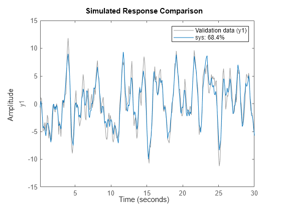
Compare the estimated output with measured data.
compare(z1,sys);

Algorithms
The general recursive prediction error algorithm (11.44) of Ljung (1999) is implemented. See also Recursive Algorithms for Online Parameter Estimation.
Version History
Introduced before R2006a