Create and Plot Identified Models Using Control System Toolbox Software

This example shows how to create and plot models using the System Identification Toolbox™ software and Control System Toolbox™ software. The example requires a Control System Toolbox license.

Construct a random numeric model using the Control System Toolbox software.

rng('default');
sys0 = drss(3,3,2);

rng('default') specifies the setting of the random number generator as its default setting.

sys0 is a third-order numeric state-space model with three outputs and two inputs.

Convert sys0 to an identified state-space model and set its output noise variance.

sys = idss(sys0);
sys.NoiseVariance = 0.1*eye(3);

Generate input data for simulating the output.

u = iddata([],idinput([800 2],'rbs'));

Simulate the model output with added noise.

opt = simOptions('AddNoise',true);
y = sim(sys,u,opt);

opt is an option set specifying simulation options. y is the simulated output for sys0.

Create an input-output ( iddata ) object.

data = [y u];

Estimate the state-space model from the generated data using ssest.

estimated_ss = ssest(data(1:400));

estimated_ss is an identified state-space model.

Convert the identified state-space model to a numeric transfer function.

sys_tf = tf(estimated_ss);

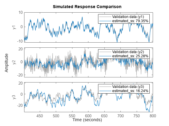
Plot the model output for identified state-space model.

compare(data(401:800),estimated_ss)

Plot the response of identified model using the Linear System Analyzer.

linearSystemAnalyzer(estimated_ss);

Related Topics

• Using Identified Models for Control Design Applications