Customize Linear Analysis Plots Using Property Editor

After you create a linear analysis response plot, you can interactively edit the plot using the Property Editor dialog box. To open the Property Editor, do one of the following:

Double-click in the plot region.
Right-click the plot, and select Properties from the context menu.

If you plot multiple responses in the same figure, you can edit the properties for each plot individually.

You can also modify response plot properties:

At the command line. For more information, see Customize Linear Analysis Plots at Command Line (Control System Toolbox).
Using the Property Inspector.

Opening the Property Editor

As an example of a response plot, consider the following step response.

sys_dc = idtf([1 4],[1 20 5]);
stepplot(sys_dc)

Overview of Property Editor

The appearance of the Property Editor dialog box depends on the type of response plot.

In general, you can change the following properties of response plots. Only the Labels and Limits tabs are available when using the Property Editor with Simulink^® Design Optimization™ software.

Titles and X- and Y-labels on the Labels tab.
Numerical ranges of the X and Y axes on the Limits tab.
Units where applicable (e.g., rad/s to Hertz) on the Units tab.
If you cannot customize units, the Property Editor displays that no units are available for the selected plot.
Styles on the Styles tab.
You can show a grid, adjust font properties, such as font size, bold, and italics, and change the axes foreground color
Change options where applicable on the Options tab.
These include peak response, settling time, phase and gain margins, etc. Plot options change with each plot response type. The Property Editor displays only the options that make sense for the selected response plot. For example, phase and gain margins are not available for step responses.

The Property Editor and its associated plot are dynamically linked. As you make changes in the Property Editor, the response plot updates immediately. Conversely, if you make changes in a plot using right-click menus, the Property Editor for that plot automatically updates.

Labels tab

To specify new text for plot titles and axis labels, type the new names in the field next to the label you want to change. The label changes immediately as you type, so you can see how the new text looks as you are typing.

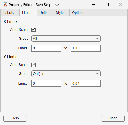
Limits tab

Default values for the axes limits make sure that the maximum and minimum x and y values are displayed. To override the default settings, change the values in the Limits fields. The Auto-Scale box automatically clears if you specify a limit value.. The new limits appear immediately in the response plot.

To reset the limits to the default values, select the Auto-Scale parameter.

For MIMO systems, you can configure different limits for each input or output. You can also use the same limits for all inputs or all outputs. In the Group drop-down lists, select:

All to specify limits for all inputs or all outputs.
An individual input or output to specify different limits. Once you specify options for a specific input or output, the corresponding limits for the All option are cleared.

Units tab

You can use the Units tab to change units in your response plot. The contents of this tab depend on the response plot associated with the editor. Use the drop-down lists to select values for each type of unit.

Response Plot	Unit Properties
Bode and Bode Magnitude	Frequency By default, shows `rad/TimeUnit` where `TimeUnit` is the system time units specified in the `TimeUnit` property of the input system. Frequency Units Options `'Hz'` `'rad/s'` `'rpm'` `'kHz'` `'MHz'` `'GHz'` `'rad/nanosecond'` `'rad/microsecond'` `'rad/millisecond'` `'rad/minute'` `'rad/hour'` `'rad/day'` `'rad/week'` `'rad/month'` `'rad/year'` `'cycles/nanosecond'` `'cycles/microsecond'` `'cycles/millisecond'` `'cycles/hour'` `'cycles/day'` `'cycles/week'` `'cycles/month'` `'cycles/year'` Frequency scale is logarithmic or linear. Magnitude in decibels (dB) or the absolute value Phase in degrees or radians
Impulse	Time By default, shows the system time units specified in the `TimeUnit` property of the input system. Time Units Options `'nanoseconds'` `'microseconds'` `'milliseconds'` `'seconds'` `'minutes'` `'hours'` `'days'` `'weeks'` `'months'` `'years'`
Nichols Chart	Frequency By default, shows `rad/TimeUnit` where `TimeUnit` is the system time units specified in the `TimeUnit` property of the input system. Frequency Units Options `'Hz'` `'rad/s'` `'rpm'` `'kHz'` `'MHz'` `'GHz'` `'rad/nanosecond'` `'rad/microsecond'` `'rad/millisecond'` `'rad/minute'` `'rad/hour'` `'rad/day'` `'rad/week'` `'rad/month'` `'rad/year'` `'cycles/nanosecond'` `'cycles/microsecond'` `'cycles/millisecond'` `'cycles/hour'` `'cycles/day'` `'cycles/week'` `'cycles/month'` `'cycles/year'` Phase in degrees or radians
Nyquist Diagram	Frequency By default, shows `rad/TimeUnit` where `TimeUnit` is the system time units specified in the `TimeUnit` property of the input system. Frequency Units Options `'Hz'` `'rad/s'` `'rpm'` `'kHz'` `'MHz'` `'GHz'` `'rad/nanosecond'` `'rad/microsecond'` `'rad/millisecond'` `'rad/minute'` `'rad/hour'` `'rad/day'` `'rad/week'` `'rad/month'` `'rad/year'` `'cycles/nanosecond'` `'cycles/microsecond'` `'cycles/millisecond'` `'cycles/hour'` `'cycles/day'` `'cycles/week'` `'cycles/month'` `'cycles/year'`
Pole/Zero Map	Time By default, shows the system time units specified in the `TimeUnit` property of the input system. Time Units Options `'nanoseconds'` `'microseconds'` `'milliseconds'` `'seconds'` `'minutes'` `'hours'` `'days'` `'weeks'` `'months'` `'years'` Frequency By default, shows `rad/TimeUnit` where `TimeUnit` is the system time units specified in the `TimeUnit` property of the input system. Frequency Units Options `'Hz'` `'rad/s'` `'rpm'` `'kHz'` `'MHz'` `'GHz'` `'rad/nanosecond'` `'rad/microsecond'` `'rad/millisecond'` `'rad/minute'` `'rad/hour'` `'rad/day'` `'rad/week'` `'rad/month'` `'rad/year'` `'cycles/nanosecond'` `'cycles/microsecond'` `'cycles/millisecond'` `'cycles/hour'` `'cycles/day'` `'cycles/week'` `'cycles/month'` `'cycles/year'`
Singular Values	Frequency By default, shows `rad/TimeUnit` where `TimeUnit` is the system time units specified in the `TimeUnit` property of the input system. Frequency Units Options `'Hz'` `'rad/s'` `'rpm'` `'kHz'` `'MHz'` `'GHz'` `'rad/nanosecond'` `'rad/microsecond'` `'rad/millisecond'` `'rad/minute'` `'rad/hour'` `'rad/day'` `'rad/week'` `'rad/month'` `'rad/year'` `'cycles/nanosecond'` `'cycles/microsecond'` `'cycles/millisecond'` `'cycles/hour'` `'cycles/day'` `'cycles/week'` `'cycles/month'` `'cycles/year'` Frequency scale is logarithmic or linear. Magnitude in decibels or the absolute value using logarithmic or linear scale
Step	Time By default, shows the system time units specified in the `TimeUnit` property of the input system. Time Units Options `'nanoseconds'` `'microseconds'` `'milliseconds'` `'seconds'` `'minutes'` `'hours'` `'days'` `'weeks'` `'months'` `'years'`

Style tab

Use the Style tab to toggle grid visibility and set font preferences and axes foreground colors for response plots.

You have the following choices:

Grid — Activate grids by default in new plots.
Fonts — Set the font size, weight (bold), and angle (italic) for fonts used in response plot titles, X/Y-labels, tick labels, and I/O names. Select font sizes from the menus or type any font-size values in the fields.
Colors — Specify the color vector to use for the axes foreground, which includes the X-Y axes, grid lines, and tick labels. Use a three-element vector to represent red, green, and blue (RGB) values. Vector element values can range from 0 to 1.
If you do not want to specify RGB values numerically, click Select to open the Color dialog box.

Options tab

The Options tab enables you to customize response characteristics for plots. Each response plot has its own set of characteristics and optional settings. When you change the value in a field, press Enter to update the response plot.

Response Characteristic Options for Response Plots

Plot	Customizable Feature
Bode Diagram and Bode Magnitude	Magnitude Response Select lower magnitude limit. Phase Response By default, plots display exact phase. Select Wrap phase to wrap the phase into the interval [–180º,180º). To wrap accumulated phase across a different interval, enter the lower limit of the interval in the text box. For example, entering 0 causes the plot to wrap the phase into the interval [0º,360º). Check Adjust phase offsets to keep phase close to a particular value, within a range of 0º–360º, at a given frequency. Confidence Region for Identified Models This option is available with System Identification Toolbox™ software. Specify number of standard deviations for plotting the response confidence region. To see the confidence region, right-click the plot, and select Characteristics > Confidence Region.
Impulse	Time Response Show settling time within xx% (specify the percentage). Confidence Region for Identified Models This option is available with System Identification Toolbox software. Number of standard deviations for display: Specify number of standard deviations for plotting the uncertainty. To see the confidence interval, right-click the plot, and select Characteristics > Confidence Region.
Nichols Chart	Magnitude Response Select lower magnitude limit. Phase Response By default, plots display exact phase. Select Wrap phase to wrap the phase into the interval [–180º,180º). To wrap accumulated phase across a different interval, enter the lower limit of the interval in the text box. For example, entering 0 causes the plot to wrap the phase into the interval [0º,360º). Check Adjust phase offsets to keep phase close to a particular value, within a range of 0º–360º, at a given frequency.
Nyquist Diagram	Confidence Region for Identified Models This option is available with System Identification Toolbox software. Number of standard deviations for display: Specify number of standard deviations for plotting the confidence ellipses. Display spacing: Specify the frequency spacing of confidence ellipses. The default is `5`, which means that the confidence ellipses are shown at every fifth frequency sample. To see the confidence ellipses, right-click the plot, and select Characteristics > Confidence Region.
Pole/Zero Map	Confidence Region for Identified Models This option is available with System Identification Toolbox software. Specify number of standard deviations for displaying the confidence region characteristic. To see the confidence region, right-click the plot, and select Characteristics > Confidence Region.
Singular Values	None
Step	Time Response Show settling time within xx% (specify the percentage). Show rise time from xx to yy% (specify the percentages) Confidence Region for Identified Models This option is available with System Identification Toolbox software. Specify number of standard deviations for plotting the response confidence region. To see the confidence region, right-click the plot, and select Characteristics > Confidence Region.