Data and Model Objects in System Identification Toolbox

Open Script

This example shows how to manage data and model objects available in the System Identification Toolbox™. System identification is about building models from data. A data set is characterized by several pieces of information: The input and output signals, the sample time, the variable names and units, and so on. Similarly, the estimated models contain information of different kinds - estimated parameters, their covariance matrices, model structure and so on.

This means that it is suitable and desirable to collect relevant information around data and models into objects. System Identification Toolbox contains a number of such objects, and the basic features of these are described in this example.

The IDDATA Object

First create some data:

u = sign(randn(200,2)); % 2 inputs
y = randn(200,1);       % 1 output
ts = 0.1;               % The sample time

To collect the input and the output in one object do

z = iddata(y,u,ts);

The data information is displayed by just typing its name:

z =

Time domain data set with 200 samples.
Sample time: 0.1 seconds               
                                       
Outputs      Unit (if specified)       
   y1                                  
                                       
Inputs       Unit (if specified)       
   u1                                  
   u2

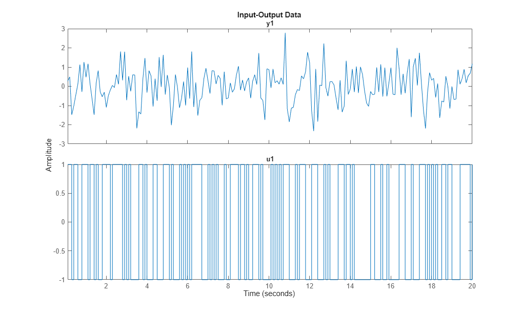
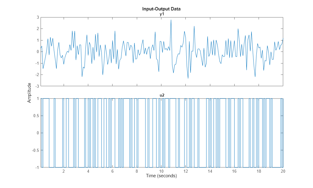
The data is plotted as iddata by the plot command, as in plot(z). Press a key to continue and advance between the subplots. Here, we plot the channels separately:

plot(z(:,1,1)) % Data subset with Input 1 and Output 1.

plot(z(:,1,2)) % Data subset with Input 2 and Output 1.

To retrieve the outputs and inputs, use

u = z.u;   % or, equivalently u = get(z,'u');
y = z.y;   % or, equivalently y = get(z,'y');

To select a portion of the data:

zp = z(48:79);

To select the first output and the second input:

zs = z(:,1,2);  % The ':' refers to all the data time points.

The sub-selections can be combined:

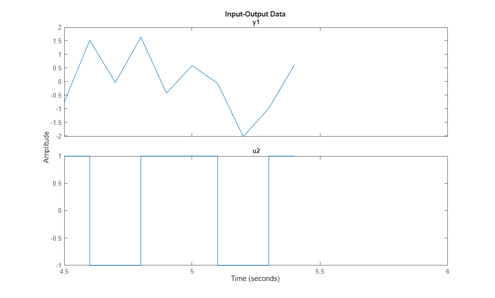
plot(z(45:54,1,2)) % samples 45 to 54 of response from second input to the first output.

The channels are given default names 'y1', 'u2', etc. This can be changed to any values by

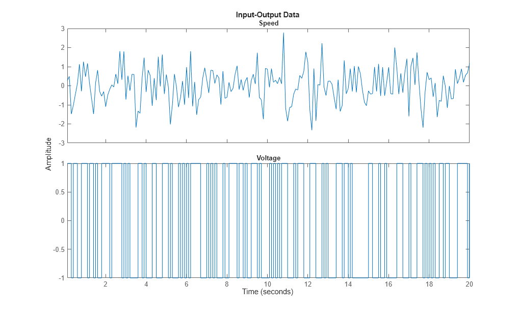
set(z,'InputName',{'Voltage';'Current'},'OutputName','Speed');

Equivalently we could write

z.inputn = {'Voltage';'Current'}; % Autofill is used for properties
z.outputn = 'Speed';    % Upper and lower cases are also ignored

For bookkeeping and plots, also units can be set:

z.InputUnit = {'Volt';'Ampere'};
z.OutputUnit = 'm/s';
z

z =

Time domain data set with 200 samples.
Sample time: 0.1 seconds               
                                       
Outputs       Unit (if specified)      
   Speed         m/s                   
                                       
Inputs        Unit (if specified)      
   Voltage       Volt                  
   Current       Ampere

All current properties are (as for any object) obtained by get:

get(z)

ans = 

  struct with fields:

              Domain: 'Time'
                Name: ''
          OutputData: [200x1 double]
                   y: 'Same as OutputData'
          OutputName: {'Speed'}
          OutputUnit: {'m/s'}
           InputData: [200x2 double]
                   u: 'Same as InputData'
           InputName: {2x1 cell}
           InputUnit: {2x1 cell}
              Period: [2x1 double]
         InterSample: {2x1 cell}
                  Ts: 0.1000
              Tstart: 0.1000
    SamplingInstants: [200x1 double]
            TimeUnit: 'seconds'
      ExperimentName: 'Exp1'
               Notes: {}
            UserData: []

In addition to the properties discussed so far, we have 'Period' which denotes the period of the input if periodic Period = inf means a non-periodic input:

z.Period

ans =

   Inf
   Inf

The intersample behavior of the input may be given as 'zoh' (zero-order-hold, i.e. piecewise constant) or 'foh' (first- order-hold, i.e., piecewise linear). The identification routines use this information to adjust the algorithms.

z.InterSample

ans =

  2x1 cell array

    {'zoh'}
    {'zoh'}

You can add channels (both input and output) by "horizontal concatenation", i.e. z = [z1 z2]:

z2 = iddata(rand(200,1),ones(200,1),0.1,'OutputName','New Output',...
    'InputName','New Input');
z3 = [z,z2]

z3 =

Time domain data set with 200 samples.
Sample time: 0.1 seconds               
                                       
Outputs          Unit (if specified)   
   Speed            m/s                
   New Output                          
                                       
Inputs           Unit (if specified)   
   Voltage          Volt               
   Current          Ampere             
   New Input

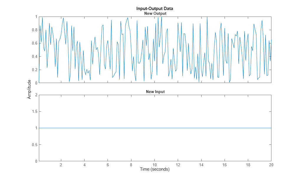
Let us plot some of the channels of z3:

plot(z3(:,1,1)) % Data subset with Input 2 and Output 1.

plot(z3(:,2,3)) % Data subset with Input 2 and Output 3.

Generating Inputs

The command idinput generates typical input signals.

u = idinput([30 1 10],'sine'); % 10 periods of 30 samples
u = iddata([],u,1,'Period',30) % Making the input an IDDATA object.

u =

Time domain data set with 300 samples.
Sample time: 1 seconds                 
                                       
Inputs       Unit (if specified)       
   u1

SIM applied to an iddata input delivers an iddata output. Let us use sim to obtain the response of an estimated model m using the input u. We also add noise to the model response in accordance with the noise dynamics of the model. We do this by using the "AddNoise" simulation option:

m = idpoly([1 -1.5 0.7],[0 1 0.5]);  % This creates a model; see below.
options = simOptions;
options.AddNoise = true;
y = sim(m,u,options) % simulated response produced as an iddata object

y =

Time domain data set with 300 samples.
Sample time: 1 seconds                 
Name: m                                
                                       
Outputs      Unit (if specified)       
   y1

The simulation input u and the output y may be combined into a single iddata object as follows:

z5 = [y u] % The output-input iddata.

z5 =

Time domain data set with 300 samples.
Sample time: 1 seconds                 
Name: m                                
                                       
Outputs      Unit (if specified)       
   y1                                  
                                       
Inputs       Unit (if specified)       
   u1

More about the iddata object is found under help iddata.

The Linear Model Objects

All models are delivered as MATLAB® objects. There are a few different objects depending on the type of model used, but this is mostly transparent.

load iddata1
m = armax(z1,[2 2 2 1]);  % This creates an ARMAX model, delivered as an IDPOLY object

All relevant properties of this model are packaged as one object (here, idpoly). To display it just type its name:

m =
Discrete-time ARMAX model: A(z)y(t) = B(z)u(t) + C(z)e(t)
  A(z) = 1 - 1.531 z^-1 + 0.7293 z^-2                    
                                                         
  B(z) = 0.943 z^-1 + 0.5224 z^-2                        
                                                         
  C(z) = 1 - 1.059 z^-1 + 0.1968 z^-2                    
                                                         
Sample time: 0.1 seconds
  
Parameterization:
   Polynomial orders:   na=2   nb=2   nc=2   nk=1
   Number of free coefficients: 6
   Use "polydata", "getpvec", "getcov" for parameters and their uncertainties.

Status:                                          
Estimated using ARMAX on time domain data "z1".  
Fit to estimation data: 76.38% (prediction focus)
FPE: 1.127, MSE: 1.082

    Many of the model properties are directly accessible

m.a    % The A-polynomial

ans =

    1.0000   -1.5312    0.7293

A list of properties is obtained by get:

get(m)

                 A: [1 -1.5312 0.7293]
                 B: [0 0.9430 0.5224]
                 C: [1 -1.0587 0.1968]
                 D: 1
                 F: 1
    IntegrateNoise: 0
          Variable: 'z^-1'
           IODelay: 0
         Structure: [1x1 pmodel.polynomial]
     NoiseVariance: 1.1045
        InputDelay: 0
       OutputDelay: 0
         InputName: {'u1'}
         InputUnit: {''}
        InputGroup: [1x1 struct]
        OutputName: {'y1'}
        OutputUnit: {''}
       OutputGroup: [1x1 struct]
             Notes: [0x1 string]
          UserData: []
              Name: ''
                Ts: 0.1000
          TimeUnit: 'seconds'
      SamplingGrid: [1x1 struct]
            Report: [1x1 idresults.polyest]

Use present to view the estimated parameter covariance as +/- 1 standard deviation uncertainty values on individual parameters:

present(m)

m =
Discrete-time ARMAX model: A(z)y(t) = B(z)u(t) + C(z)e(t)        
  A(z) = 1 - 1.531 (+/- 0.01801) z^-1 + 0.7293 (+/- 0.01473) z^-2
                                                                 
  B(z) = 0.943 (+/- 0.06074) z^-1 + 0.5224 (+/- 0.07818) z^-2    
                                                                 
  C(z) = 1 - 1.059 (+/- 0.06067) z^-1 + 0.1968 (+/- 0.05957) z^-2
                                                                 
Sample time: 0.1 seconds
  
Parameterization:
   Polynomial orders:   na=2   nb=2   nc=2   nk=1
   Number of free coefficients: 6
   Use "polydata", "getpvec", "getcov" for parameters and their uncertainties.

Status:                                                       
Termination condition: Near (local) minimum, (norm(g) < tol)..
Number of iterations: 3, Number of function evaluations: 7    
                                                              
Estimated using ARMAX on time domain data "z1".               
Fit to estimation data: 76.38% (prediction focus)             
FPE: 1.127, MSE: 1.082                                        
More information in model's "Report" property.

Use getpvec to fetch a flat list of all the model parameters, or just the free ones, and their uncertainties. Use getcov to fetch the entire covariance matrix.

[par, dpar] = getpvec(m, 'free')
CovFree = getcov(m,'value')

par =

   -1.5312
    0.7293
    0.9430
    0.5224
   -1.0587
    0.1968


dpar =

    0.0180
    0.0147
    0.0607
    0.0782
    0.0607
    0.0596


CovFree =

    0.0003   -0.0003    0.0000    0.0007    0.0004   -0.0003
   -0.0003    0.0002   -0.0000   -0.0004   -0.0003    0.0002
    0.0000   -0.0000    0.0037   -0.0034   -0.0000    0.0001
    0.0007   -0.0004   -0.0034    0.0061    0.0008   -0.0005
    0.0004   -0.0003   -0.0000    0.0008    0.0037   -0.0032
   -0.0003    0.0002    0.0001   -0.0005   -0.0032    0.0035

nf = 0, nd = 0 denote orders of a general linear model, of which the ARMAX model is a special case.

Report contains information about the estimation process:

m.Report
m.Report.DataUsed       % record of data used for estimation
m.Report.Fit            % quantitative measures of model quality
m.Report.Termination    % search termination conditions

ans = 

              Status: 'Estimated using ARMAX with prediction focus'
              Method: 'ARMAX'
    InitialCondition: 'zero'
                 Fit: [1x1 struct]
          Parameters: [1x1 struct]
         OptionsUsed: [1x1 idoptions.polyest]
           RandState: [1x1 struct]
            DataUsed: [1x1 struct]
         Termination: [1x1 struct]


ans = 

  struct with fields:

            Name: 'z1'
            Type: 'Time domain data'
          Length: 300
              Ts: 0.1000
     InterSample: 'zoh'
     InputOffset: []
    OutputOffset: []


ans = 

  struct with fields:

    FitPercent: 76.3807
       LossFcn: 1.0824
           MSE: 1.0824
           FPE: 1.1266
           AIC: 887.1256
          AICc: 887.4123
          nAIC: 0.1192
           BIC: 909.3483


ans = 

  struct with fields:

                 WhyStop: 'Near (local) minimum, (norm(g) < tol).'
              Iterations: 3
    FirstOrderOptimality: 7.2436
                FcnCount: 7
              UpdateNorm: 0.0067
         LastImprovement: 0.0067

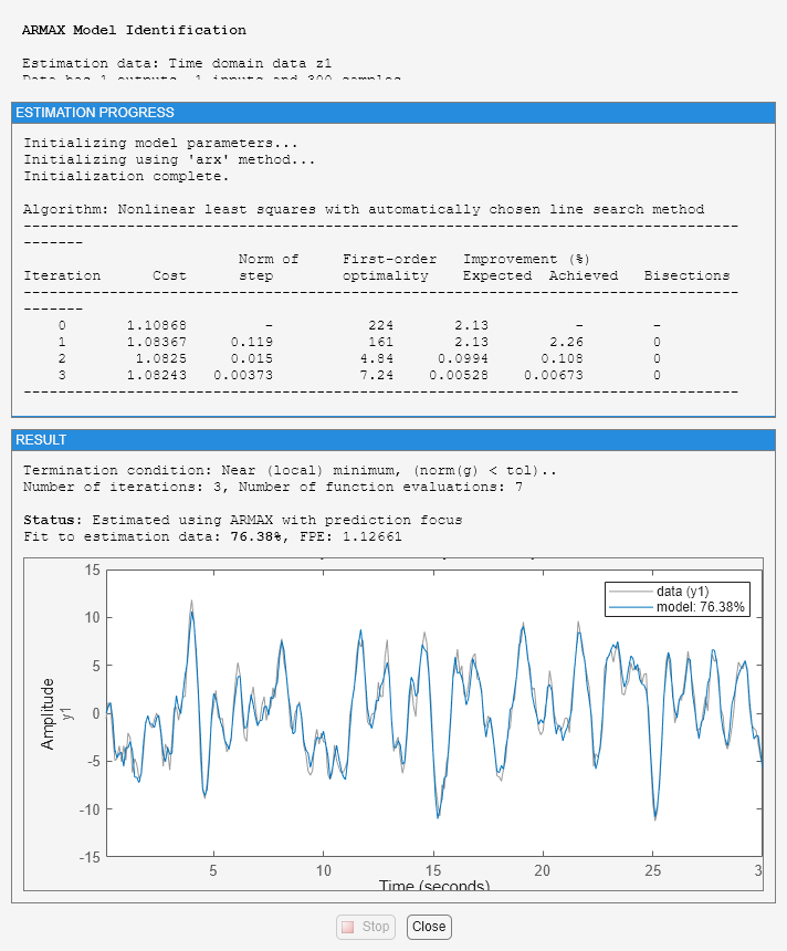
To obtain on-line information about the minimization, use the 'Display' estimation option with possible values 'off', 'on', and 'full'. This launches a progress viewer that shows information on the model estimation progress.

Opt = armaxOptions('Display','on');
m1 = armax(z1,[2 2 2 1],Opt);

Variants of Linear Models - IDTF, IDPOLY, IDPROC, IDSS and IDGREY

There are several types of linear models. The one above is an example of the idpoly version for polynomial type models. Different variants of polynomial-type models, such as Box-Jenkins models, Output Error models, ARMAX models etc are obtained using the corresponding estimators - bj, oe, armax, arx etc. All of these are presented as idpoly objects.

Other variants are idss for state-space models; idgrey for user-defined structured state-space models; idtf for transfer function models, and idproc for process models (gain+delay+static gain).

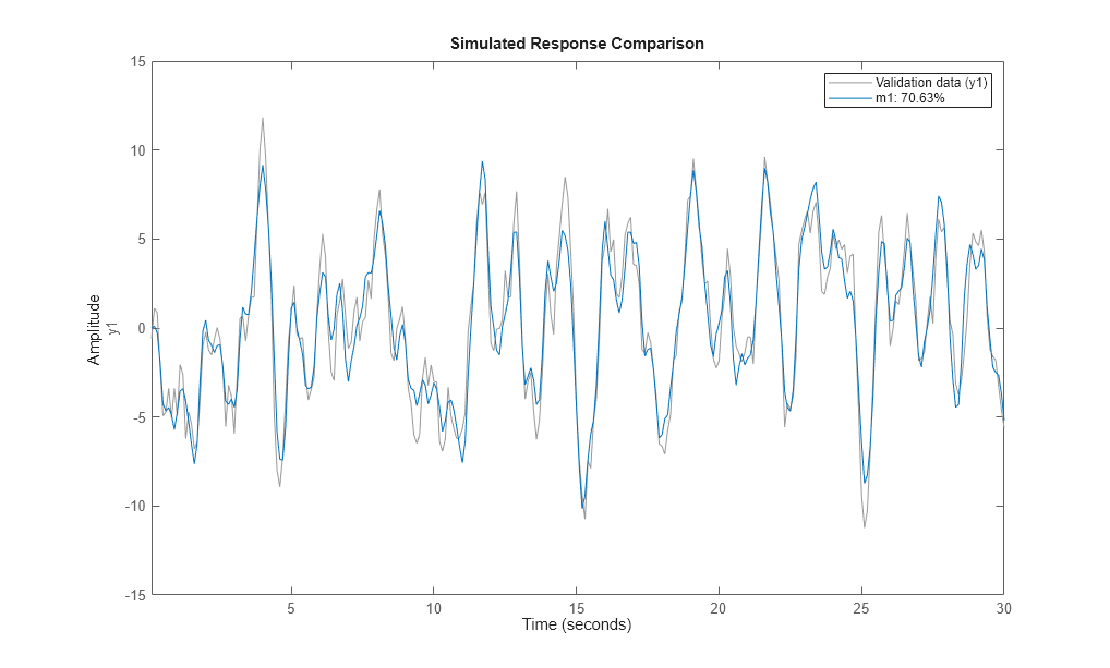
The commands to evaluate the model: bode, step, iopzmap, compare, etc, all operate directly on the model objects, for example:

compare(z1,m1)

Transformations to state-space, transfer function and zeros/poles are obtained by idssdata, tfdata and zpkdata:

[num,den]  = tfdata(m1,'v')

num =

         0    0.9430    0.5224


den =

    1.0000   -1.5312    0.7293

The 'v' means that num and den are returned as vectors and not as cell arrays. The cell arrays are useful to handle multivariable systems. To also retrieve the 1 standard deviation uncertainties in the values of num and den use:

[num, den, ~, dnum, dden] = tfdata(m1,'v')

num =

         0    0.9430    0.5224


den =

    1.0000   -1.5312    0.7293


dnum =

         0    0.0607    0.0782


dden =

         0    0.0180    0.0147

Transforming Identified Models into Numeric LTIs of Control System Toolbox

The objects also connect directly to the Control System Toolbox™ model objects, like tf, ss, and zpk, and can be converted into these LTI objects, if Control System Toolbox is available. For example, tf converts an idpoly object into a tf object.

CSTBInstalled = exist('tf','class')==8;
if CSTBInstalled % check if Control System Toolbox is installed
    tfm = tf(m1) % convert IDPOLY model m1 into a TF object
end

tfm =
 
  From input "u1" to output "y1":
    0.943 z^-1 + 0.5224 z^-2
  ----------------------------
  1 - 1.531 z^-1 + 0.7293 z^-2
 
Sample time: 0.1 seconds
Discrete-time transfer function.

When converting an IDLTI model to the Control Systems Toolbox's LTI models, noise component is not retained. To also include the noise channels as regular inputs of the LTI model, use the 'augmented' flag:

if CSTBInstalled
    tfm2 = tf(m1,'augmented')
end

tfm2 =
 
  From input "u1" to output "y1":
    0.943 z^-1 + 0.5224 z^-2
  ----------------------------
  1 - 1.531 z^-1 + 0.7293 z^-2
 
  From input "v@y1" to output "y1":
  1.051 - 1.113 z^-1 + 0.2069 z^-2
  --------------------------------
    1 - 1.531 z^-1 + 0.7293 z^-2
 
Input groups:           
      Name      Channels
    Measured       1    
     Noise         2    
                        
Sample time: 0.1 seconds
Discrete-time transfer function.

The noise channel is named v@y1 in the model tfm2.