Dealing with Multi-Experiment Data and Merging Models
R2026bThis example shows how to deal with multiple experiments and merge models when working with System Identification Toolbox™ for estimating and refining models.
Introduction
The analysis and estimation functions in System Identification Toolbox let you work with multiple batches of data. Essentially, if you have performed multiple experiments and recorded several input-output datasets, you can group them up into a single iddata object and use them with any estimation routine.
In some cases, you can "split up" your (single) measurement dataset to remove portions where the data quality is not good. For example, a portion of the data may be unusable due to external disturbance or sensor failure. In those cases, you can separate out each good portion of data and then combine them into a single multi-experiment iddata object.
For example, look at the dataset iddemo8data.mat.
load iddemo8dataView the data object, dat.
dat
dat =

Time domain data set with 1000 samples.
Sample time: 1 seconds

Outputs      Unit (if specified)
   y1

Inputs       Unit (if specified)
   u1

Data Properties
plot(dat)
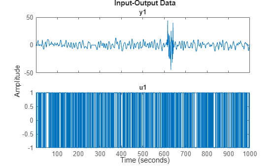
You can see that there are some problems with the output around samples 250 to 280 and around samples 600 to 650. These could have been sensor failures.
Therefore, split the data into three separate experiments and put them into a multi-experiment data object.
d1 = dat(1:250);
d2 = dat(281:600);
d3 = dat(651:1000);
d = merge(d1,d2,d3) % merge lets you create multi-exp iddata object
d =
Time domain data set containing 3 experiments.
Experiment Samples Sample Time
Exp1 250 1
Exp2 320 1
Exp3 350 1
Outputs Unit (if specified)
y1
Inputs Unit (if specified)
u1
Data Properties
You can give different names to the different experiments.
d.ExperimentName = {'Period 1';'Day 2';'Phase 3'}d =
Time domain data set containing 3 experiments.
Experiment Samples Sample Time
Period 1 250 1
Day 2 320 1
Phase 3 350 1
Outputs Unit (if specified)
y1
Inputs Unit (if specified)
u1
Data Properties
To examine the multi-experiment data object, use the plot command (plot(d)).
Performing Estimation Using Multi-Experiment Data
As mentioned before, all model estimation routines accept multi-experiment data and take into account that they are recorded at different periods. Use the first two experiments for estimation and the third one for validation.
de = getexp(d,[1,2]);      % subselection is done using the command getexp
dv = getexp(d,'Phase 3');  % using numbers or names
m1 = arx(de,[2 2 1]);
m2 = n4sid(de,2);
m3 = armax(de,[2 2 2 1]);
compare(dv,m1,m2,m3)
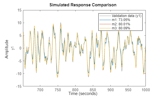
The compare command also accepts multiple experiments. Use the right-click menu to pick the experiment to use, one at a time.
compare(d,m1,m2,m3)
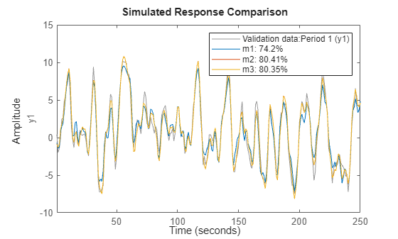
Also, spa, etfe, resid, predict, and sim operate in the same way for multi-experiment data, as they do for single experiment data.
Representing Multi-Experiment Data Using Matrices and Timetables
Instead of using iddata object, you can equivalently represent the multi-experiment data using a cell array of numeric matrices and timetables.
tt1 = timetable(seconds(d1.SamplingInstants),d1.u,d1.y);
tt2 = timetable(seconds(d2.SamplingInstants),d2.u,d2.y);
m1_mat = arx({d1.u,d2.u},{d1.y,d2.y},[2 2 1]);
m1_tt = arx({tt1,tt2},[2 2 1]);
compare(dv,m1,m1_mat,m1_tt)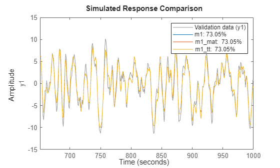
Merging Models After Estimation
There is another way to deal with separate data sets. You can compute a model for each set and then merge the models.
m4 = armax(getexp(de,1),[2 2 2 1]);
m5 = armax(getexp(de,2),[2 2 2 1]);
m6 = merge(m4,m5); % m4 and m5 are merged into m6
This is conceptually the same as computing m from the merged set de, but not numerically the same. Working on de assumes that the signal-to-noise ratios are (about) the same in the different experiments, while merging separate models makes independent estimates of the noise levels. If the conditions are about the same for the different experiments, it is more efficient to estimate directly on the multi-experiment data.
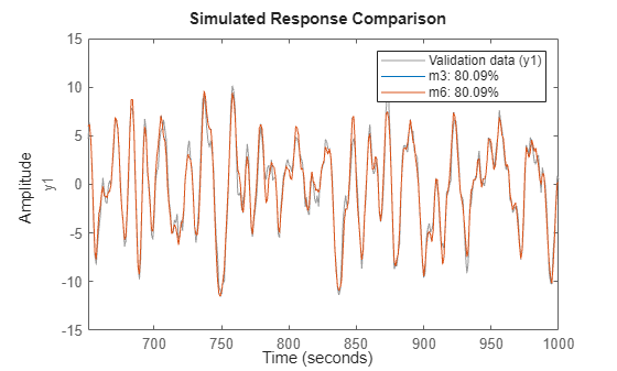
You can check the models m3 and m6, that are both ARMAX models obtained on the same data in two different ways.
[m3.a;m6.a]
ans = 2×3

    1.0000    -1.5034    0.7008
    1.0000    -1.5022    0.7000
[m3.b;m6.b]
ans = 2×3

    0    1.0023    0.5029
    0    1.0035    0.5028
[m3.c;m6.c]
ans = 2×3

    1.0000    -0.9744    0.1578
    1.0000    -0.9751    0.1584
compare(dv,m3,m6)
Case Study: Concatenating vs. Merging Independent Datasets
Now consider two data sets generated by the system m0.
m0
m0 =
  Discrete-time identified state-space model:
    x(t+Ts) = A x(t) + B u(t) + K e(t)
       y(t) = C x(t) + D u(t) + e(t)

  A =
             x1        x2        x3
   x1    0.5296    -0.476    0.1238
   x2    -0.476  -0.09743    0.1354
   x3    0.1238    0.1354   -0.8233

  B =
             u1        u2
   x1    -1.146  -0.03763
   x2     1.191    0.3273
   x3         0         0

  C =
            x1       x2       x3
   y1  -0.1867  -0.5883  -0.1364
   y2   0.7258        0   0.1139

  D =
          u1     u2
   y1  1.067      0
   y2      0      0

  K =
       y1  y2
   x1   0   0
   x2   0   0
   x3   0   0

Sample time: 1 seconds

Parameterization:
   STRUCTURED form (some fixed coefficients in  A, B, C).
   Feedthrough: on some input channels
   Disturbance component: none
   Number of free coefficients: 23
   Use "idssdata", "getpvec", "getcov" for parameters and their uncertainties.

Status:
Created by direct construction or transformation. Not estimated.

Model Properties
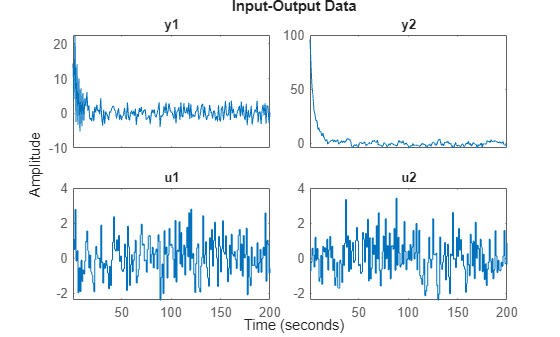
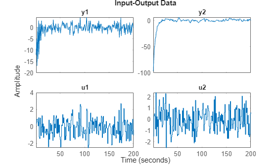
You collect the data sets z1 and z2, obtained from m0 with different inputs, noise and initial conditions. You obtain these datasets from iddemo8data.mat that was loaded earlier.
Plot the first data set.
plot(z1)
Plot the second data set.
plot(z2)
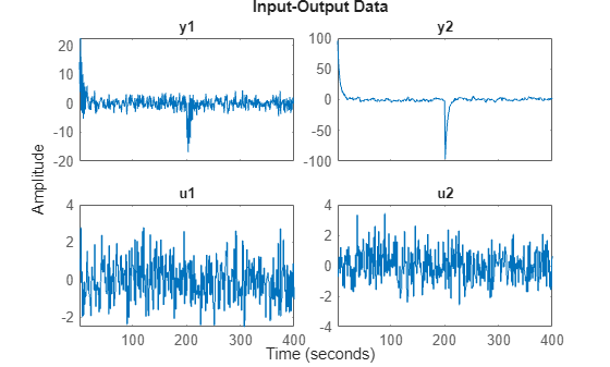
Concatenate the data obtained and plot it.
zzl = [z1;z2]
zzl =

Time domain data set with 400 samples.
Sample time: 1 seconds

Outputs      Unit (if specified)
   y1
   y2

Inputs       Unit (if specified)
   u1
   u2

Data Properties
plot(zzl)
You can obtain a discrete-time state-space model using ssest.
ml = ssest(zzl,3,'Ts',1,'Feedthrough', [true, false]);
Compare the bode response for the models m0 and ml.
clf
bode(m0,ml)
legend('show')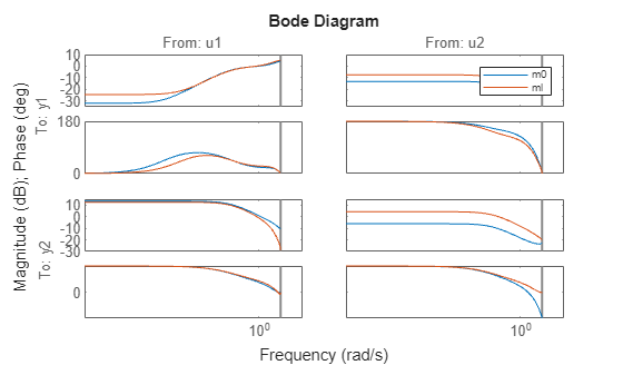
This is not a very good model, as observed from the four Bode plots above.
Now, treat the two data sets as different experiments.
zzm = merge(z1,z2)
zzm =
Time domain data set containing 2 experiments.

Experiment   Samples      Sample Time
   Exp1         200            1
   Exp2         200            1

Outputs      Unit (if specified)
   y1
   y2

Inputs       Unit (if specified)
   u1
   u2

Data Properties
% The model for this data can be estimated as before (watching progress this time)
mm = ssest(zzm,3,'Ts',1,'Feedthrough',[true, false], ssestOptions('Display', 'on'));
Compare the bode plots of the true system (blue), the model from concatenated data (green), and the model from the merged data set (red).
clf
bode(m0,'b',ml,'g',mm,'r')
legend('show')
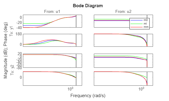
The merged data set gives a better model, as observed from the plot above.
Identifying Linear Models Using Multi-Experiment Data
When identifying a linear model using multi-experiment data, you estimate the initial condition separately for each experiment. You can find this information in the report.
mm.Report.Parameters.X0
ans = 3×2

     1.4243    -1.4165
    -0.0138     0.0607
    -0.8412     0.8619
Conclusions
This example analyzes the use of multiple data sets together for the estimation of one model. This technique is useful when you have multiple datasets from independent experiment runs or when you segment data into multiple sets to remove bad segments. You can package multiple experiments into a single iddata object, a cell array of numeric matrices, or a cell array of timetables, which is then usable for all estimation and analysis requirements. This technique works for both time and frequency domain data.
You can also merge models after estimation. You can use this technique to "average out" independently estimated models. If the noise characteristics on multiple datasets are different, merging models after estimation works better than merging the datasets themselves before estimation.

