分析多变量系统中的数据并辨识模型
此示例展示如何处理具有多个输入和输出通道的数据(MIMO 数据)。重点介绍了常见操作,例如查看 MIMO 数据、估计和比较模型以及查看相应的模型响应。
数据集
我们首先查看数据集 SteamEng。
load SteamEng该数据集是从实验室规模的蒸汽机收集的。它具有控制阀后的蒸汽(实际上是压缩空气)的 Pressure 输入,以及连接到输出轴的发电机上的 Magnetization voltage 输入。
输出是发电机中的 Generated voltage 和发电机的 Rotational speed(产生的交流电压的频率)。采样时间为 50 毫秒。
首先将测量的通道收集到 iddata 对象中:
steam = iddata([GenVolt,Speed],[Pressure,MagVolt],0.05);
steam.InputName = {'Pressure';'MagVolt'};
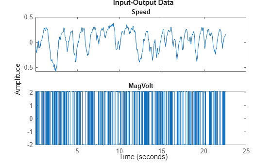
steam.OutputName = {'GenVolt';'Speed'};让我们来看看这些数据。
plot(steam(:,1,1))

plot(steam(:,1,2))
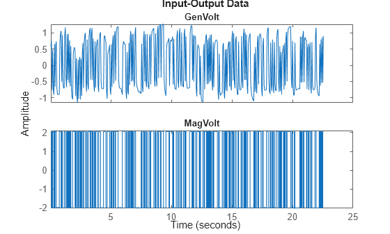
plot(steam(:,2,1))

plot(steam(:,2,2))
阶跃响应与冲激响应
感受动态的第一步是查看直接从数据估计的不同通道之间的阶跃响应:
mi = impulseest(steam,50);
clf, step(mi)

带有置信域的响应
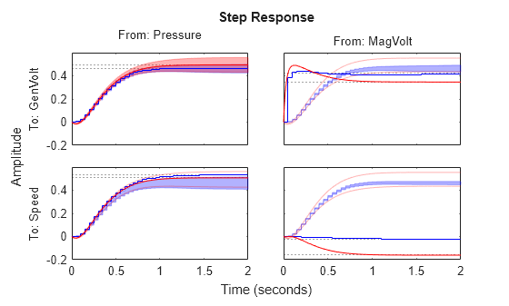
为了查看响应的重要性,可以使用冲激图,其置信域对应于 3 个标准差:
showConfidence(impulseplot(mi),3)

显然,非对角线影响占主导地位。(比较 y 刻度!)也是说,GenVolt 主要受 MagVolt 的影响(动态不大),而 Speed 主要依赖于 Pressure。显然 MagVolt 对 Speed 的回应并不十分显著。
双输入双输出模型
快速的首次测试也是查看默认的连续时间状态空间预测误差模型。仅使用前半部分数据进行估计:
mp = ssest(steam(1:250))
mp =
  Continuous-time identified state-space model:
      dx/dt = A x(t) + B u(t) + K e(t)
       y(t) = C x(t) + D u(t) + e(t)

  A =
            x1       x2       x3       x4
   x1   -29.43   -4.561   0.5994     -5.2
   x2   0.4848  -0.8662   -4.101   -2.336
   x3    2.839    5.084   -8.566   -3.855
   x4   -12.13   0.9224    1.818   -34.29

  B =
       Pressure   MagVolt
   x1    0.1033    -1.617
   x2   -0.3027  -0.09415
   x3    -1.566    0.2953
   x4  -0.04477    -2.681

  C =
                 x1       x2       x3       x4
   GenVolt   -16.39   0.3767  -0.7566    2.808
   Speed     -5.623    2.246  -0.5356    3.423

  D =
            Pressure   MagVolt
   GenVolt         0         0
   Speed           0         0

  K =
       GenVolt    Speed
   x1  -0.3555   0.0853
   x2  -0.0231    5.195
   x3    1.526    2.132
   x4    1.787  0.03216

Parameterization:
   FREE form (all coefficients in A, B, C free).
   Feedthrough: none
   Disturbance component: estimate
   Number of free coefficients: 40
   Use "idssdata", "getpvec", "getcov" for parameters and their uncertainties.

Status:
Estimated using SSEST on time domain data.
Fit to estimation data: [86.9;74.84]% (prediction focus)
FPE: 3.897e-05, MSE: 0.01414

Model Properties
与直接从数据估计的阶跃响应进行比较:
h = stepplot(mi,'b',mp,'r',2); % Blue for direct estimate, red for mp
showConfidence(h)
一致性良好,且变化在所示的置信边界内是允许的。
为了测试状态空间模型的质量,在未用于估计的数据部分上仿真并比较输出:
compare(steam(251:450),mp)

该模型非常擅长重现验证数据的生成电压,并且速度也相当合理。(使用下拉菜单查看不同输出的适合情况。)
频谱分析
类似地,将 mp 的频率响应与频谱分析估计值进行比较,可以得出:
msp = spa(steam);
bode(msp,mp)
clf
bode(msp,'b',mp,'r')
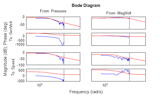
您可以右键点击该图并选择不同的 I/O 对以仔细查看。您还可以选择“特征:置信域' 用于表示波特图可靠性的图片。
和以前一样,MagVolt 对 Speed 的回应并不显著,而且难以估计。
单输入单输出 (SISO) 模型
该数据集很快就给出了良好的模型。否则,您经常必须尝试某些渠道的子模型才能看到显著的影响。工具箱对象为此类工作中必要的簿记提供了全面支持。输入和输出名称是其中的核心。
阶跃响应表明 MagVolt 主要影响 GenVolt,而 Pressure 主要影响 Speed。为此构建两个简单的 SISO 模型。选择频道时可以使用名称和号码。
m1 = tfest(steam(1:250,'Speed','Pressure'),2,1); % TF model with 2 poles 1 zero
m2 = tfest(steam(1:250,1,2),1,0) % Simple TF model with 1 pole.
m2 =

  From input "MagVolt" to output "GenVolt":
    18.57
  ---------
  s + 43.53

Continuous-time identified transfer function.

Parameterization:
   Number of poles: 1   Number of zeros: 0
   Number of free coefficients: 2
   Use "tfdata", "getpvec", "getcov" for parameters and their uncertainties.

Status:
Estimated using TFEST on time domain data.
Fit to estimation data: 73.34%
FPE: 0.04645, MSE: 0.04535

Model Properties
将这些模型与 MIMO 模型 mp 进行比较:
compare(steam(251:450),m1,m2,mp)

SISO 模型与完整模型相比效果良好。现在让我们比较一下奈奎斯特图。m1 是蓝色,m2 是绿色,mp 是红色。请注意,排序是自动的。mp 描述所有输入输出对,而 m1 仅包含 Pressure 到 Speed,m2 仅包含 MagVolt 到 GenVolt。
clf
showConfidence(nyquistplot(m1,'b',m2,'g',mp,'r'),3)

SISO 模型可以很好地重现各自的输出。
经验法则是,当您添加更多输出(更多解释!)时,模型拟合会变得更加困难,而当您添加更多输入时,模型拟合会变得更加简单。
双输入单输出模型
为了更好地完成输出 GenVolt,可以使用两个输入。
m3 = armax(steam(1:250,'GenVolt',:),'na',4,'nb',[4 4],'nc',2,'nk',[1 1]);
m4 = tfest(steam(1:250,'GenVolt',:),2,1);
compare(steam(251:450),mp,m3,m4,m2)

与仅使用 Pressure 作为输入的 m3 相比,通过在模型 m4(离散时间)和 m2(连续时间)中包含输入 MagVolt 可以实现约 10% 的改进。
合并 SISO 模型
如果需要,可以通过首先创建零虚拟模型将两个 SISO 模型 m1 和 m2 组合成一个“非对角线”模型:
mdum = idss(zeros(2,2),zeros(2,2),zeros(2,2),zeros(2,2));
mdum.InputName = steam.InputName;
mdum.OutputName = steam.OutputName;
mdum.ts = 0; % Continuous time model
m12 = [idss(m1),mdum('Speed','MagVolt')];    % Adding Inputs.
                                             % From both inputs to Speed
m22 = [mdum('GenVolt','Pressure'),idss(m2)]; % Adding Inputs.
                                             % From both inputs to GenVolt

mm = [m12;m22]; % Adding the outputs to a 2-by-2 model.

compare(steam(251:450),mp,mm)

显然,“非对角线”模型 mm 在解释输出方面表现得与 m1 和 m2 类似。