Linear Approximation of Complex Systems by Identification
R2026bThis example shows how to obtain linear approximations of a complex, nonlinear system by means of linear model identification. The approach is based on selection of an input signal that excites the system. A linear approximation is obtained by fitting a linear model to the simulated response of the nonlinear model for the chosen input signal.
This example uses Simulink®, Control System Toolbox™ and Simulink Control Design™.
Introduction
In many situations, a linear model is obtained by simplification of a more complex nonlinear system under certain local conditions. For example, a high fidelity model of the aircraft dynamics may be described by a detailed Simulink model. A common approach taken to speed up the simulation of such systems, study their local behavior about an operating point or design compensators is to linearize them. If we perform the linearization of the original model analytically about an operating point, this, in general, would yield a model of an order as high as, or close to, the number of states in the original model. This order may be unnecessarily high for the class of inputs it is supposed to be used with for analysis or control system design. Hence we can consider an alternative approach centered around collecting input-output data from the simulation of the system and using it to derive a linear model of just the right order.
Analytical Linearization of F14 Model
Consider the F14 model. This is already a linear model but contains derivative blocks and sources of disturbance that may affect the nature of its output. We can "linearize" it between its one input port and the two output ports as follows:
open_system('idF14Model')
IO = getlinio('idF14Model')
syslin = linearize('idF14Model',IO)
3x1 vector of Linearization IOs:
--------------------------
1. Linearization input perturbation located at the following signal:
- Block: idF14Model/Pilot
- Port: 1
- Signal Name: Stick Input
2. Linearization output measurement located at the following signal:
- Block: idF14Model/Gain5
- Port: 1
- Signal Name: Angle of Attack
3. Linearization output measurement located at the following signal:
- Block: idF14Model/Pilot G force
- Port: 1
- Signal Name: Pilot G force

syslin =

  A =
                 Transfer Fcn    Derivative  Transfer Fcn   Derivative1
   Transfer Fcn       -0.6385             0         689.4             0
   Derivative               1        -1e+05             0             0
   Transfer Fcn      -0.00592             0       -0.6571             0
   Derivative1              0             0             1        -1e+05
   Actuator Mod             0             0         1.424             0
   Alpha-sensor      0.001451             0             0             0
   Stick Prefil             0             0             0             0
   Pitch Rate L             0             0             1             0
   Proportional             0             0       -0.8156             0

                 Actuator Mod  Alpha-sensor  Stick Prefil  Pitch Rate L
   Transfer Fcn         -1280             0             0             0
   Derivative               0             0             0             0
   Transfer Fcn        -137.7             0             0             0
   Derivative1              0             0             0             0
   Actuator Mod           -20         2.986        -39.32         -1.67
   Alpha-sensor             0        -2.526             0             0
   Stick Prefil             0             0        -22.52             0
   Pitch Rate L             0             0             0        -4.144
   Proportional             0         -1.71         22.52        0.9567

                 Proportional
   Transfer Fcn             0
   Derivative               0
   Transfer Fcn             0
   Derivative1              0
   Actuator Mod        -3.864
   Alpha-sensor             0
   Stick Prefil             0
   Pitch Rate L             0
   Proportional             0

  B =
                 Stick Input
   Transfer Fcn            0
   Derivative              0
   Transfer Fcn            0
   Derivative1             0
   Actuator Mod            0
   Alpha-sensor            0
   Stick Prefil            1
   Pitch Rate L            0
   Proportional            0

  C =
                 Transfer Fcn    Derivative  Transfer Fcn   Derivative1
   Angle of Att      0.001451             0             0             0
   Pilot G forc         -3106     3.106e+08     7.083e+04    -7.081e+09

                 Actuator Mod  Alpha-sensor  Stick Prefil  Pitch Rate L
   Angle of Att             0             0             0             0
   Pilot G forc             0             0             0             0

                 Proportional
   Angle of Att             0
   Pilot G forc             0

  D =
                 Stick Input
   Angle of Att            0
   Pilot G forc            0

Continuous-time state-space model.
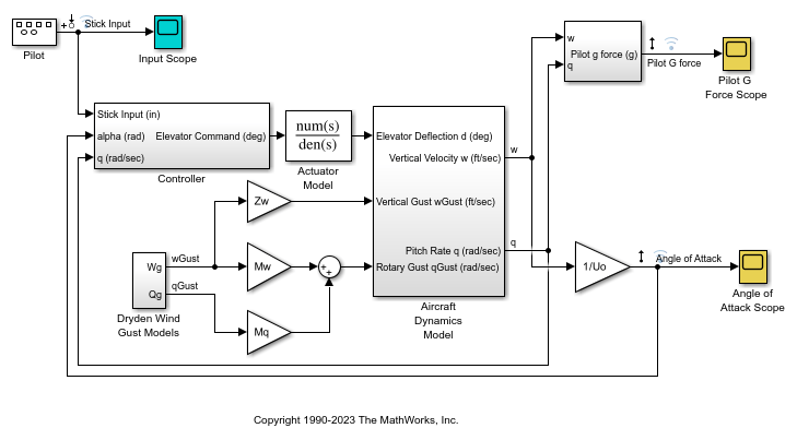
syslin is a model with 2 outputs, one input and 9 states. This is because the linearization path from the "Stick Input" input to the two outputs has 9 states in the original system. We can verify this by using operpoint:
operpoint('idF14Model')
ans =


 Operating point for the Model idF14Model.
 (Time-Varying Components Evaluated at time t=0)

States:
----------
x
_

(1.) idF14Model/Actuator Model
0
(2.) idF14Model/Aircraft Dynamics Model/Transfer Fcn.1
0
(3.) idF14Model/Aircraft Dynamics Model/Transfer Fcn.2
0
(4.) idF14Model/Controller/Alpha-sensor Low-pass Filter
0
(5.) idF14Model/Controller/Pitch Rate Lead Filter
0
(6.) idF14Model/Controller/Proportional plus integral compensator
0
(7.) idF14Model/Controller/Stick Prefilter
0
(8.) idF14Model/Dryden Wind Gust Models/Q-gust model
0
(9.) idF14Model/Dryden Wind Gust Models/W-gust model
0
0

Inputs: None
----------
Could this order be reduced while still maintaining fidelity to the responses for the chosen square-wave ("Stick input") input?
Preparing Identification Data
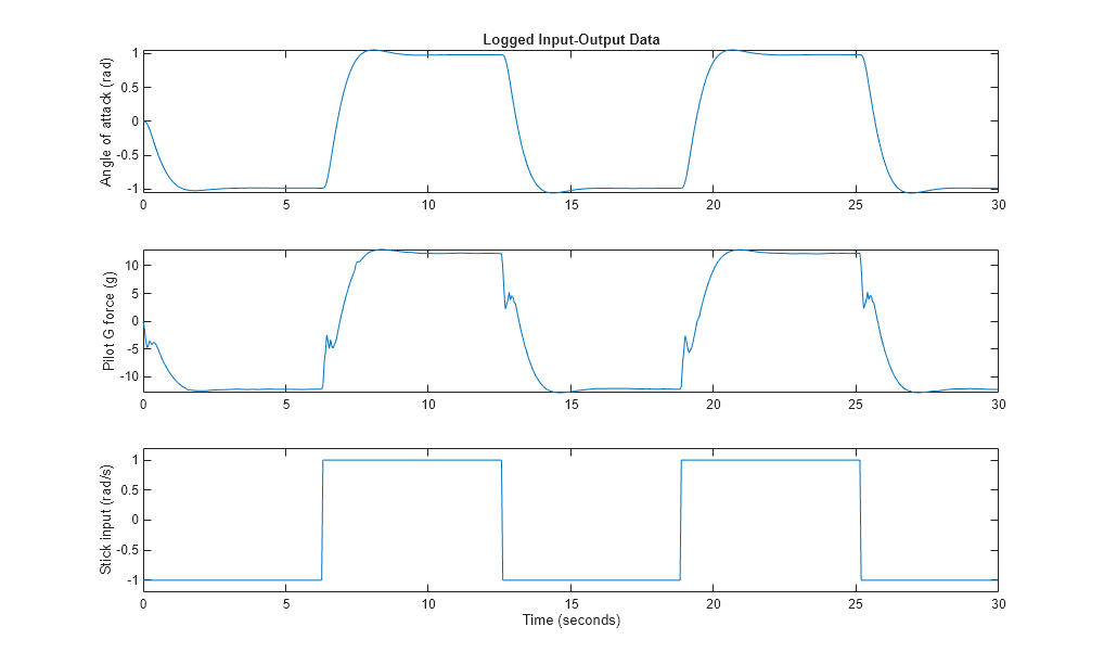
Simulate the model and log the input square wave (u) and the outputs "Angle of attack" (y1) and "Pilot G force" (y2) for 0:30 second time span. This data, after interpolation to a uniformly spaced time vector (sample time of 0.0444 seconds), is stored in the "idF14SimData.mat" file.
load idF14SimData
Z = iddata([y1, y2],u,Ts,'Tstart',0);
Z.InputName = 'Stick input'; Z.InputUnit = 'rad/s';
Z.OutputName = {'Angle of attack', 'Pilot G force'};
Z.OutputUnit = {'rad', 'g'};
t = Z.SamplingInstants;

subplot(311)
plot(t,Z.y(:,1)), ylabel('Angle of attack (rad)')
title('Logged Input-Output Data')

subplot(312)
plot(t,Z.y(:,2)), ylabel('Pilot G force (g)')

subplot(313)
plot(t,Z.u), ylabel('Stick input (rad/s)')
axis([0 30 -1.2 1.2])
xlabel('Time (seconds)')
Estimation of State Space Models
Estimate state-space models of orders 2 to 4 using the ssest command. We configure the estimation to use "simulation" focus and choose to not estimate the disturbance component of the model.
opt = ssestOptions('Focus','simulation');
syslin2 = ssest(Z, 2, 'DisturbanceModel', 'none', opt);
syslin3 = ssest(Z, 3, 'DisturbanceModel', 'none', opt);
syslin4 = ssest(Z, 4, 'DisturbanceModel', 'none', opt);
Compare the performance of the linearized model syslin and the three identified models to the data. Note that syslin is an SS model while syslin2, syslin3 and syslin4 are IDSS models.
syslin.InputName = Z.InputName;
syslin.OutputName = Z.OutputName; % reconcile names to facilitate comparison
clf
compare(Z, syslin, syslin2, syslin3, syslin4)
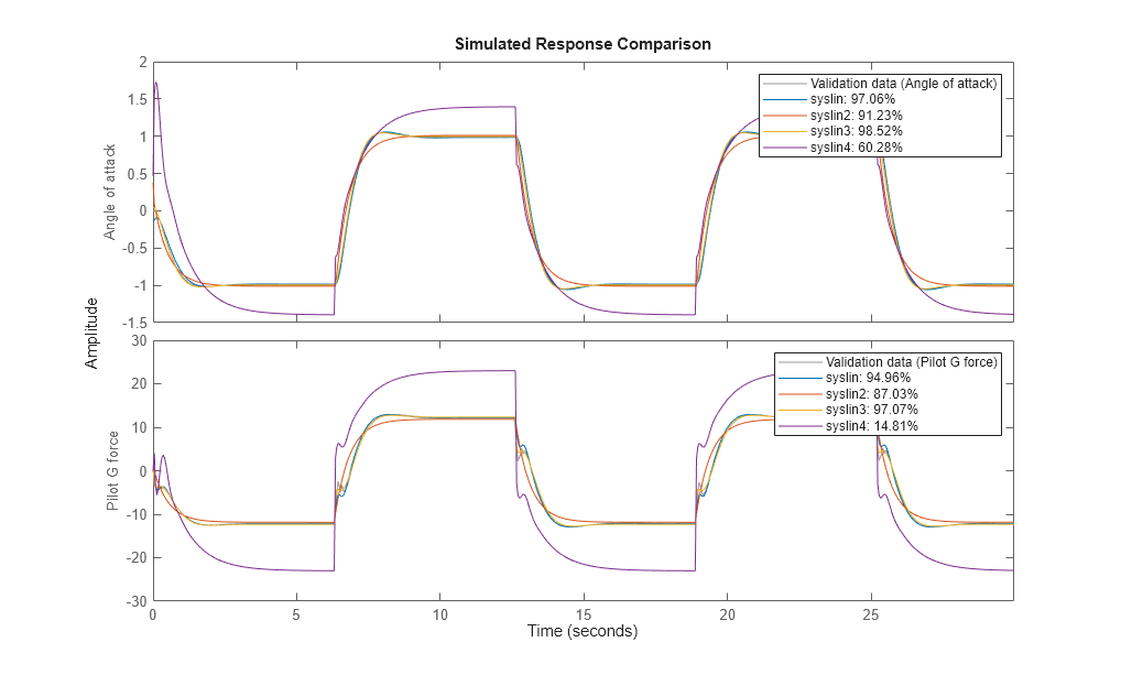
The plot shows that the 3rd order model (syslin3) works pretty well as a linear approximation of aircraft dynamic about its default (t=0) operating conditions. It fits the data slightly better than the one obtained by analytical linearization (syslin). If the original idF14Model is linear, why doesn't its linearization result, syslin, produce a 100% fit to the data? There are two reasons for this:
The measured outputs are affected by the wind gusts which means that the logged outputs are not simply a function of the Stick input. There are disturbances affecting it.
The "Pilot G force" block uses derivative blocks whose linearization depends upon the value of the time constant "c". "c" should be small (we use 1e-5) but not zero. A non-zero value for c introduces an approximation error in the linearization.
Let us view the parameters of the model syslin3 which seems to capture the responses pretty well:
syslin3
syslin3 =
  Continuous-time identified state-space model:
      dx/dt = A x(t) + B u(t) + K e(t)
       y(t) = C x(t) + D u(t) + e(t)

  A =
           x1      x2      x3
   x1  -1.006   2.029  0.5842
   x2  -8.284  -19.39   5.611
   x3   2.784   12.63  -6.956

  B =
       Stick input
   x1       0.2614
   x2       -5.512
   x3        3.606

  C =
                     x1      x2      x3
   Angle of att  -8.841  0.5347   1.402
   Pilot G forc  -86.42   15.85   66.12

  D =
                 Stick input
   Angle of att            0
   Pilot G forc            0

  K =
       Angle of att  Pilot G forc
   x1             0             0
   x2             0             0
   x3             0             0

Parameterization:
   FREE form (all coefficients in A, B, C free).
   Feedthrough: none
   Disturbance component: none
   Number of free coefficients: 18
   Use "idssdata", "getpvec", "getcov" for parameters and their uncertainties.

Status:
Estimated using SSEST on time domain data "Z".
Fit to estimation data: [98.4;97.02]%
FPE: 2.367e-05, MSE: 0.1103
Model Simplification by Reduction and Estimation
We can also take the approach of reducing the order of the linearized model syslin and refining the parameters of the reduced model to best fit the data Z. To figure out a good value for the reduced order, we use hsvd:
[S, BalData] = hsvd(syslin);
clf; bar(S)
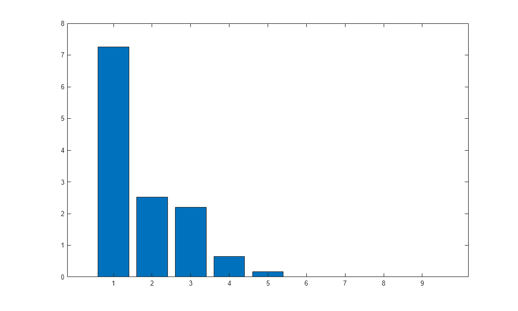
The bar chart shows that the singular values are quite small for states 4 and above. Hence 3rd order might be optimal for reduction.
sysr = balred(syslin,3,BalData)
opt2 = bodeoptions; opt2.PhaseMatching = 'on';
clf; bodeplot(sysr,syslin,opt2)
sysr =

  A =
            x1       x2       x3
   x1   -2.854    -7.61   -54.04
   x2  -0.9714    2.341    9.123
   x3   0.6979   -7.203   -24.08

  B =
       Stick input
   x1       -137.7
   x2         -869
   x3       -506.7

  C =
                         x1          x2          x3
   Angle of att  -0.0005063  -0.0008826   -0.001016
   Pilot G forc   -0.005926    -0.04692     -0.1646

  D =
                 Stick input
   Angle of att     -0.03784
   Pilot G forc       -1.617

Continuous-time state-space model.
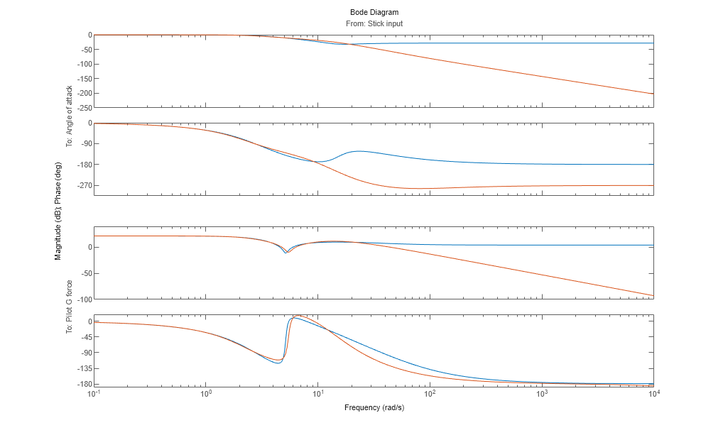
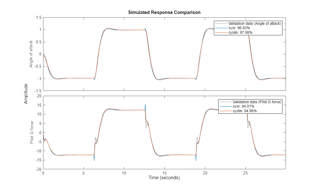
The bode plot shows good fidelity up to 10 rad/s. sysr is able to emulate the responses as good as the original 9-state model as shown by the compare plot:
compare(Z, sysr, syslin)
Let us refine the parameters of sysr to improve its fit to data. For this estimation, we choose the "Levenberg-Marquardt" search method and change the maximum number of allowable iterations to 10. These choices were made based on some trial and error. We also turn on the display of estimation progress.
opt.Display = 'on';
opt.SearchMethod = 'lm';
opt.SearchOptions.MaxIterations = 10;
sysr2 = ssest(Z, sysr, opt)
compare(Z, sysr2)
sysr2 =
  Continuous-time identified state-space model:
      dx/dt = A x(t) + B u(t) + K e(t)
       y(t) = C x(t) + D u(t) + e(t)

  A =
            x1       x2       x3
   x1   -4.048   -7.681   -54.01
   x2  -0.4844    1.549    8.895
   x3  -0.2398   -6.777   -25.78

  B =
       Stick input
   x1       -137.7
   x2         -869
   x3       -506.7

  C =
                         x1          x2          x3
   Angle of att  -0.0003361  -0.0004964     0.00215
   Pilot G forc    -0.01191    -0.03599     -0.1434

  D =
                 Stick input
   Angle of att     0.003022
   Pilot G forc       0.6438

  K =
       Angle of att  Pilot G forc
   x1             0             0
   x2             0             0
   x3             0             0

Parameterization:
   FREE form (all coefficients in A, B, C free).
   Feedthrough: yes
   Disturbance component: none
   Number of free coefficients: 20
   Use "idssdata", "getpvec", "getcov" for parameters and their uncertainties.

Status:
Estimated using SSEST on time domain data "Z".
Fit to estimation data: [98.78;97.03]%
FPE: 1.434e-05, MSE: 0.1097
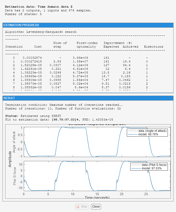
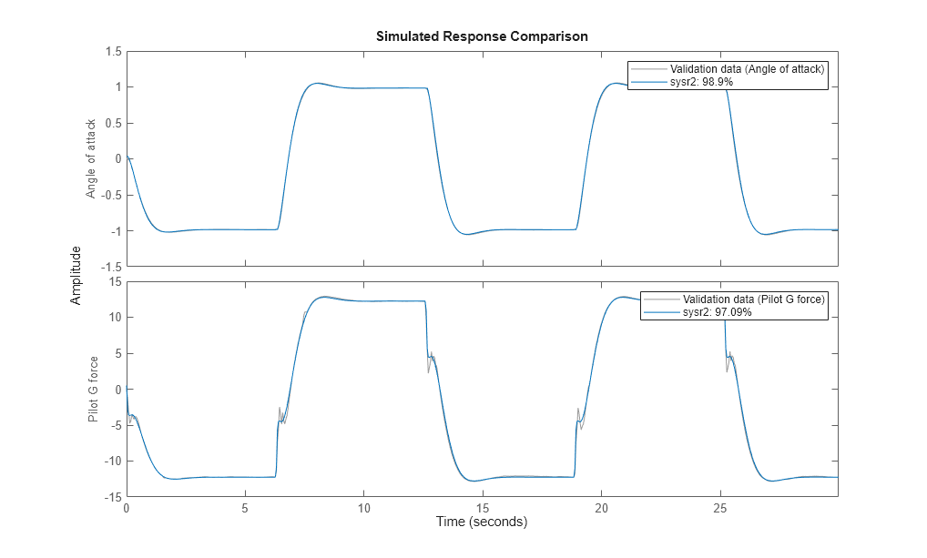
The refined model sysr2 fits the response of the F14 model quite well (about 99% for the first output, and about 97% for the second).
Conclusions
We showed an alternative approach to analytical linearization for obtaining linear approximations of complex systems. The results are derived for a particular input signal and, strictly speaking, are applicable to that input only. To improve the applicability of results to various input profiles, we could perform several simulations using the various types of inputs. We could then merge the resulting datasets into one multi-experiment dataset (see iddata/merge) and use it for estimations. In this example, we used a complex, but linear system for convenience. The real benefit of this approach would be seen for nonlinear systems.
We also showed an approach for reducing the order of a linear system while keeping the reduced model faithful to the simulated response of the original Simulink model. The role of the reduced model sysr was to provide an initial guess for the estimated model sysr2. The approach also highlights the fact that any linear system, including those of a different class, can be used as the initial model for estimations.
bdclose('idF14Model')

