Piezoelectric Actuator Model Identification Using Machine Learning

Experimental Setup

The data used in this example was provided by Prof. Micky Rakotondrabe (University of Toulouse, France) who performed the experiment in a laboratory in University of Franche-Comté at Besançon, France.

The experimental setup consists of a cantilevered piezoelectric actuator that is used in precise positioning applications. The actuator has two layers, namely, a piezoelectric layer that is made of lead zirconate titanate and a passive layer that is made of nickel. Piezoelectric actuators are used in several applications including high precision positioning and inkjet printing.

Identification of Piezoelectric Actuators

Piezoelectric actuators suffer from several problems, including hysteresis, creep, and vibration. Models based on physical principles must take these characteristics into account. The identification process for piezoelectric actuator models usually involves estimating a mathematical model that combines a nonlinear component that characterizes the behavior of the hysteresis with a linear model that characterizes the linear dynamics of the actuator. This example uses two approaches that are based on machine learning to identify a black box model of a piezoelectric actuator. The example assumes that there is no prior knowledge about the dynamics of the actuator or the hysteresis nonlinearity.

Input-Output Data

The input v is the voltage [V] applied to the actuator and the output d is the displacement of the actuator [$\mu$m]. The data set contains 10,000 input-output samples corresponding to a sampling rate of 0.0002 s. This data will be used for all estimation and validation tasks carried out in this example.

% load data
load idPiezoElectricData.mat

Estimation and Validation Data

The input voltage applied to the piezoelectric actuator in this data set is a summation of sinusoidal signals with different frequencies. The data set is split into two parts, ze and zv, where the first 5000 samples are used for estimation (ze), and the remaining 5000 samples are used for validation (zv).

ze = idPiezoElectricData(1:5000);   % estimation data
zv = idPiezoElectricData(5001:end); % validation data

Plot the two data sets together to visually verify their time ranges.

figure; plot(ze, zv);
legend('ze','zv');

Identification Using Nonlinear ARX Model with Support Vector Machine Output Function

Configure a support vector machine (SVM) function to represent the nonlinearity in the system model.

Create the regressor set Regressors to use in the template idnlarx model.

Vars = {'d', 'v'};                           
Lags = {1:20, 0:20};

Regressors = linearRegressor(Vars, Lags);  

Configure the idSupportVectorMachine nonlinearity object NL.

NL = idSupportVectorMachine;
NL.EpsilonMargin = 1e-3;
NL.KernelScale = 30;

Create a template idnlarx model initialModel that incorporates Regressors and NL. Then use initialModel to estimate an NLARX model mdlSVM from the data ze.

initialModel = idnlarx(ze.OutputName, ze.InputName, Regressors, NL);  
mdlSVM = nlarx(ze, initialModel);    

Visualize how the estimated model compares with the validation data.

compare(zv,mdlSVM);

The legend in the figure shows a high fit accuracy for this model.

Identification Using Nonlinear ARX Model with Gaussian Process Output Function

Configure a Gaussian process (GP) function to represent the nonlinearity in the system model.

Create the regressor set Regressors to use in the template idnlarx model.

% Create Regressors                                                       
Vars = {'d','v'};
Lags = {1:5,0:5};
Regressors = linearRegressor(Vars, Lags);

Configure the idGaussianProcess nonlinearity object NL.

NL = idGaussianProcess;    

Create a template idnlarx model initialModel that incorporates Regressors and NL. Then use initialModel to estimate an NLARX model mdlGP from the data ze.

initialModel = idnlarx(ze.OutputName, ze.InputName, Regressors, NL);
mdlGP = nlarx(ze, initialModel);

Visualize how the estimated model compares with the validation data.

compare(zv,mdlGP);

The legend in the figure shows a high fit accuracy for this model.

Compare Results for Nonlinear Models and Linear Model

Compare the identified models obtained using nonlinear ARX with support vector machines and Gaussian process output functions to an identified linear model obtained using the ssest command.

First set options for ssest using the option set ssestOptions. Then estimate a linear model mdlLinear using ssest.

opt = ssestOptions;
opt.EnforceStability = true;
opt.Focus = 'simulation';
mdlLinear = ssest(ze,6,opt);

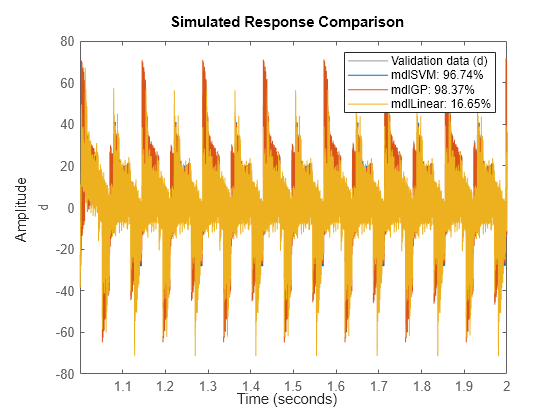
Visualize how the three estimated models compare with the validation data.

figure 
compare(zv,mdlSVM,mdlGP,mdlLinear);

The legend in the figure shows that the fit accuracy obtained using a linear model is significantly lower than the fit accuracies for both nonlinear ARX models with output functions based on machine learning.