Nonlinear Modeling of a Magneto-Rheological Fluid Damper
This example shows nonlinear black-box modeling of the dynamic behavior of a magneto-rheological fluid damper. It shows how to create Nonlinear ARX and Hammerstein-Wiener models of the damper using measurements of its velocity and the damping force.
The data used in this example was provided by Dr. Akira Sano (Keio University, Japan) and Dr. Jiandong Wang (Peking University, China) who performed the experiments in a laboratory of Keio University. See the following reference for a more detailed description of the experimental system and some related studies.
J.Wang, A. Sano, T. Chen, and B. Huang. Identification of Hammerstein systems without explicit parameterization of nonlinearity. International Journal of Control, In press, 2008. DOI: 10.1080/00207170802382376.
Experimental Setup
Magneto-Rheological (MR) fluid dampers are semi-active control devices used for reducing vibrations of various dynamic structures. MR fluids, whose viscosities depend on the input voltage/current of the device, provide controllable damping forces.
To study the behavior of such devices, a MR damper was fixed at one end to the ground and connected at the other end to a shaker table generating vibrations. The voltage of the damper was set to 1.25 v. The damping force f(t) was sampled every 0.005 s. The displacement was sampled every 0.001 s, which was then used to estimate the velocity v(t) at the sampling period of 0.005 s.
Input-Output Data
A data set containing the input and output measurements was stored in a MAT file called mrdamper.mat. The input v(t) is the velocity [cm/s] of the damper, and the output f(t) is the damping force [N]. The MAT file contains 3499 samples of data corresponding to a sampling rate of 0.005 s. This data will be used for all the estimation and validation tasks carried out in this example.
% Let us begin by loading and inspecting the data.
load('mrdamper.mat');
who
Your variables are:

F   Ts  V
Package loaded variables F (output force), V (input velocity) and Ts (sample time) into an IDDATA object.
z = iddata(F, V, Ts, 'Name', 'MR damper', ...
    'InputName', 'v', 'OutputName', 'f',...
    'InputUnit', 'cm/s', 'OutputUnit', 'N');
Data Preparation for Estimation and Validation
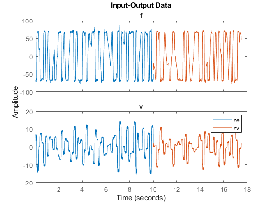
Split this data set z into two subsets, first 2000 samples to be used for estimation (ze), and the rest to be used for validation of results (zv).
ze = z(1:2000);    % estimation data
zv = z(2001:end);  % validation data
Let us plot the two data sets together to visually verify their time ranges:
plot(ze, zv)
legend('ze','zv')
Model Order Selection
The first step in estimating black box models is to choose model orders. The definition of orders depends upon the type of model.
For linear and nonlinear ARX models, the orders are represented by three numbers: na, nb and nk which define the number of past outputs, past inputs and input delays used for predicting the value of output at a given time. The set of time-delayed I/O variables defined by the orders are called "regressors". For more flexibility in creating regressors, you can use the regressor specification objects (see linearRegressor, polynomialRegressor, customRegressor).
For Hammerstein-Wiener models, which represent linear models with static I/O nonlinearities, the orders define the number of poles and zeros and input delay of the linear component. They are defined by numbers nb (number of zeros +1), nf (number of poles), and nk (input delay in number of lags).
Typically model orders are chosen by trial and error. However, the orders of the linear ARX model may be computed automatically using functions such as arxstruc and selstruc. The orders thus obtained give a hint about the possible orders to use for the nonlinear models as well. So let us first try to determine the best order for a linear ARX model.
V = arxstruc(ze,zv,struc(1:5, 1:5,1:5)); % try values in the range 1:5 for na, nb, nk
Order = selstruc(V,'aic') % selection of orders by Akaike's Information Criterion
Order =

     2     4     1
The AIC criterion has selected Order = [na nb nk] = [2 4 1], meaning that in the selected ARX model structure, damper force f(t) is predicted by the 6 regressors f(t-1), f(t-2), v(t-1), v(t-2), v(t-3) and v(t-4).
For more information on model order selection, see the example titled "Model Structure Selection: Determining Model Order and Input Delay".
Preliminary Analysis: Creating Linear Models
It is advisable to try linear models first because they are simpler to create. If linear models do not provide satisfactory results, the results provide a basis for exploration of nonlinear models.
Let us estimate linear ARX and Output-Error (OE) models of orders suggested by output of SELSTRUC above.
LinMod1 = arx(ze, [2 4 1]); % ARX model Ay = Bu + e
LinMod2 = oe(ze, [4 2 1]);  % OE model  y = B/F u + e
Similarly, we may create a linear state-space model whose order (= number of states) will be determined automatically:
LinMod3 = ssest(ze); % creates a state-space model of order 3
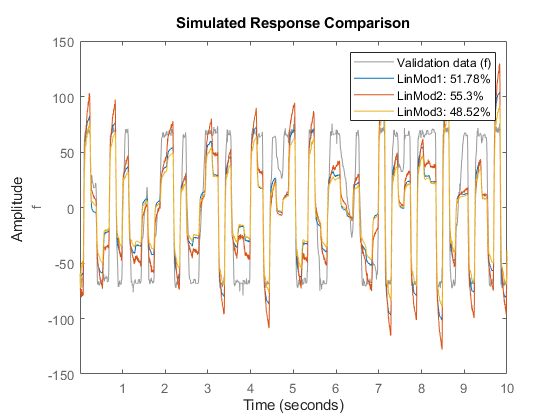
Let us now compare the responses of these models to the measured output data in ze:
compare(ze, LinMod1, LinMod2, LinMod3) % comparison to estimation data
A better test for model quality is to validate it against an independent data set. Hence we compare the model responses against data set zv.
compare(zv, LinMod1, LinMod2, LinMod3) % comparison to validation data
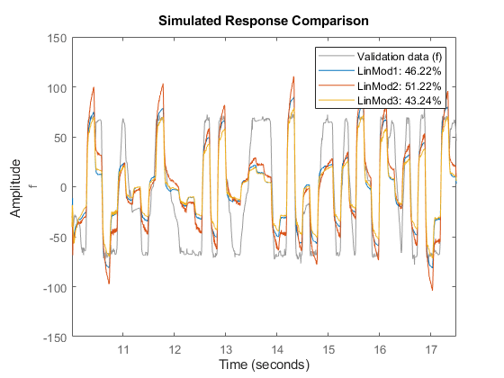
As observed, the best of these linear models has a fit of 51% on the validation data set.
Creating Nonlinear ARX Models
The linear model identification revealed that an ARX model provided less than 50% fit to the validation data. To achieve better results we now explore the use of Nonlinear ARX (IDNLARX) models. The need for nonlinear models for this data is also suggested by the advice utility which may be used to inspect data for potential advantage of using a nonlinear model over a linear model.
advice(ze, 'nonlinearity')
There is an indication of nonlinearity in the data.
A nonlinear ARX model of order [4 4 1] and idTreePartition function performs
better prediction of output than the corresponding ARX model of the same order.
Consider using nonlinear models, such as IDNLARX, or IDNLHW. You may also use
the "isnlarx" command to test for nonlinearity with more options.
The Nonlinear ARX models can be considered as nonlinear counterparts of ARX models that provide greater modeling flexibility by two means:
The regressors may be combined using a nonlinear function rather than a weighted sum employed by ARX models. Nonlinear functions such as sigmoid network, binary tree and wavelet network may be used. In the identification context, these functions are called "nonlinear mapping functions".
The regressors can themselves be arbitrary (possibly nonlinear) functions of I/O variables in addition to time-delayed variable values employed by ARX models.
Creating Regressors for Nonlinear ARX Models
When linear with contiguous lags, the regressors are most easily created using order matrix [na nb nk], as described above. In the most general case of regressors with arbitrary lags, or when the regressors are based on the absolute values of the variables, using the linearRegressor object provides more flexibility. In case the regressors are polynomials of time-delayed variables, they can be created using the polynomialRegressor object. For regressors employing arbitrary, user-specified formulas, customRegressor objects may be used.
We will explore using various model orders and using various nonlinear mapping functions. Use of polynomial or custom regressors is not explored. For ways of specifying custom regressors in IDNLARX models, see the example titled "Building Nonlinear ARX Models with Nonlinear and Custom Regressors".
Estimating a Default Nonlinear ARX Model
To begin, let us estimate an IDNLARX model of order [2 4 1] and a sigmoid network as the type of nonlinearity. We shall use MaxIterations = 50, and Levenberg-Marquardt search method as estimation options for all estimations below.
Options = nlarxOptions('SearchMethod', 'lm');
Options.SearchOptions.MaxIterations = 50;
Narx1 = nlarx(ze, [2 4 1], idSigmoidNetwork, Options)
Narx1 =

<strong>Nonlinear ARX model with 1 output and 1 input</strong>
  Inputs: v
  Outputs: f

Regressors:
  Linear regressors in variables f, v

Output function: Sigmoid network with 10 units
Sample time: 0.005 seconds

Status:
Estimated using NLARX on time domain data "MR damper".
Fit to estimation data: 95.8% (prediction focus)
FPE: 6.648, MSE: 6.08
nlarx is the command used for estimating Nonlinear ARX models. Narx1 is a Nonlinear ARX model with regressors R := [f(t-1), f(t-2), v(t-1) ... v(t-4)]. The nonlinearity is a Sigmoid network that uses a combination of sigmoid unit functions and a linear weighted sum of regressors to compute the output. The mapping function is stored in the OutputFcn property of the model.
disp(Narx1.OutputFcn)
<strong>Sigmoid Network</strong>
Inputs: f(t-1), f(t-2), v(t-1), v(t-2), v(t-3), v(t-4)
Output: f(t)

 Nonlinear Function: Sigmoid network with 10 units
 Linear Function: initialized to [48.3 -3.38 -3.34 -2.7 -1.38 2.15]
 Output Offset: initialized to -21.4

    NonlinearFcn: '<Sigmoid units and their parameters>'
       LinearFcn: '<Linear function parameters>'
          Offset: '<Offset parameters>'
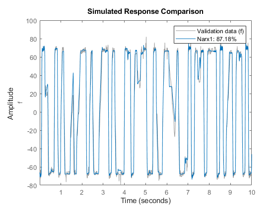
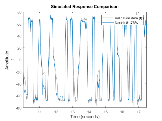
Examine the model quality by comparing the simulated output against the estimated and validated data sets ze and zv:
compare(ze, Narx1); % comparison to estimation data
compare(zv, Narx1); % comparison to validation data
Trying Various Model Orders
We see a better fit as compared to the linear models of same orders. Next, we can try other orders in the vicinity of those suggested by SELSTRUC.
NL = idSigmoidNetwork;
Narx2{1} = nlarx(ze, [3 4 1], NL, Options); % use na = 3, nb = 4, nk = 1.
Narx2{1}.Name = 'Narx2_1';
Narx2{2} = nlarx(ze, [2 5 1], NL, Options); Narx2{2}.Name = 'Narx2_2';
Narx2{3} = nlarx(ze, [3 5 1], NL, Options); Narx2{3}.Name = 'Narx2_3';
Narx2{4} = nlarx(ze, [1 4 1], NL, Options); Narx2{4}.Name = 'Narx2_4';
Narx2{5} = nlarx(ze, [2 3 1], NL, Options); Narx2{5}.Name = 'Narx2_5';
Narx2{6} = nlarx(ze, [1 3 1], NL, Options); Narx2{6}.Name = 'Narx2_6';
Evaluate the performance of these models on estimation and validation data sets:
compare(ze, Narx1, Narx2{:}); % comparison to estimation data
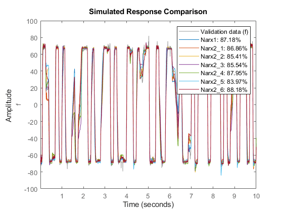
compare(zv, Narx1, Narx2{:}); % comparison to validation data
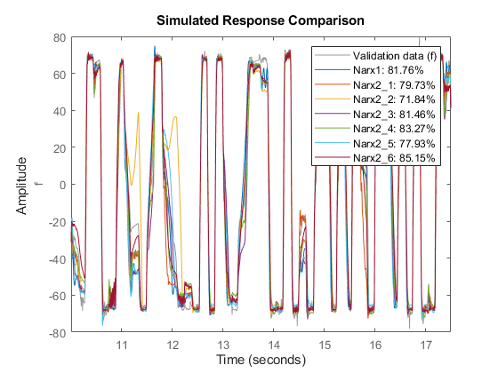
The model Narx2{6} seems to be providing good fits to both estimation and validation data sets while its orders are smaller than those of Narx1. Based on this observation, let us use [1 3 1] as orders for subsequent trials, and retain Nlarx2{6} for fit comparisons. This choice of orders corresponds to using [f(t-1), v(t-1), v(t-2), v(t-3)] as the set of regressors.
Specifying Number of Units for Sigmoid Network Function
Next, let us explore the structure of the Sigmoid Network function. The most relevant property of this estimator is the number of sigmoid units it uses. Create one that uses 12 sigmoid units.
Sig = idSigmoidNetwork(12); % create a network that uses 12 units
Narx3 = nlarx(ze, [1 3 1], Sig, Options);
We compare this model against Narx1 and Narx2{6}, on estimation and validation data sets:
compare(ze, Narx3, Narx1, Narx2{6}); % comparison to estimation data
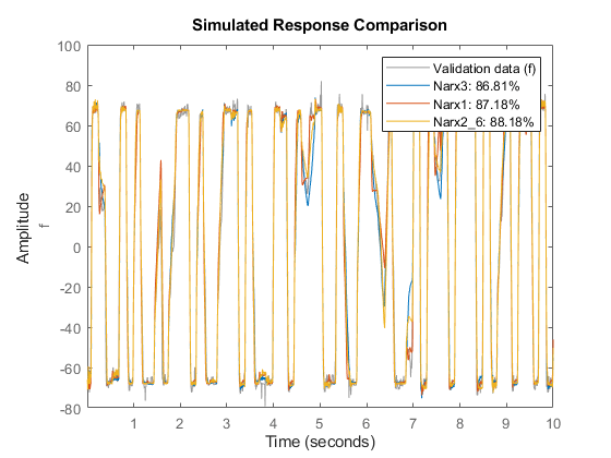
compare(zv, Narx3, Narx1, Narx2{6}); % comparison to validation data
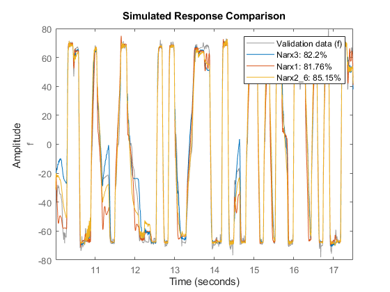
The new model Narx3 provides no better fit than Narx2{6}. Hence we retain the number of units to 10 in subsequent trials.
Choosing Regressor Subset for Nonlinear Mapping Function
Typically, all the regressors defined by chosen orders ([1 3 1] here) are used by the nonlinear function (sigmoid network). If the number of regressors is large, this may increase the model complexity. It is possible to select a subset of regressors to be used by the components of the sigmoid network without modifying the model orders. This is facilitated by the property called 'RegressorUsage'. Its value is a table that specifies which regressors are used by which components. For example, we may explore using only those regressors that are contributed by the input variables to be used by the nonlinear component of the sigmoid function. This can be done as follows:
Sig = idSigmoidNetwork(10);
NarxInit = idnlarx(ze.OutputName, ze.InputName, [1 3 1], Sig);
NarxInit.RegressorUsage.("f:NonlinearFcn")(1) = false;
disp(NarxInit.RegressorUsage)
Narx4 = nlarx(ze, NarxInit, Options);
              f:LinearFcn    f:NonlinearFcn
              ___________    ______________

    f(t-1)       true            false
    v(t-1)       true            true
    v(t-2)       true            true
    v(t-3)       true            true
This causes the regressors v(t-1), v(t-2), and v(t-3) to be used by the sigmoid unit functions. The output variable based regressor f(t-1) is not used. Note that the idSigmoidNetwork function also contains a linear term represented by a weighted sum of all regressors. The linear term uses the full set of regressors.
Create another model that uses regressors {y1(t-1), u1(t-2), u1(t-3)} for its nonlinear component.
Use = false(4,1);
Use([1 3 4]) = true;
NarxInit.RegressorUsage{:,2} = Use;
Narx5 = nlarx(ze, NarxInit, Options);
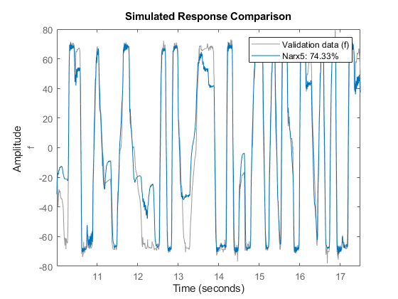
The model Narx5 seems to perform very well for both estimation and validation data sets.
compare(ze, Narx5); % comparison to estimation data
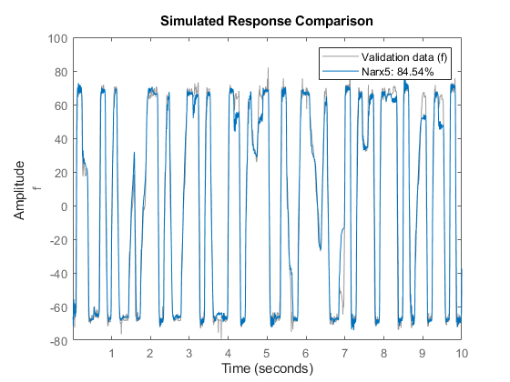
compare(zv, Narx5); % comparison to validation data
Trying Various Nonlinear Mapping Functions
So far we have explored various model orders, number of units to be used in the Sigmoid Network function and specification of a subset of regressors to be used by the nonlinear component of the sigmoid network. Next, we try using other types of nonlinear functions.
Use a Wavelet Network function with default properties. Like the sigmoid network, a wavelet network maps the regressors to the output by using a sum of linear and nonlinear components; the nonlinear component uses a sum of wavelets.
NarxInit = idnlarx(ze.OutputName, ze.InputName, [1 3 1], idWaveletNetwork);
% Use only regressors 1 and 3 for the nonlinear component of network
NarxInit.RegressorUsage.("f:NonlinearFcn")([2 4]) = false;
Narx6 = nlarx(ze, NarxInit, Options);
Use a Tree Partition nonlinear function with 20 units:
TreeNet = idTreePartition;
TreeNet.NonlinearFcn.NumberOfUnits = 20;
NarxInit.OutputFcn = TreeNet;
Narx7 = nlarx(ze, NarxInit, Options);
Compare the results against Narx3 and Narx5
compare(ze, Narx3, Narx5, Narx6, Narx7) % comparison to estimation data
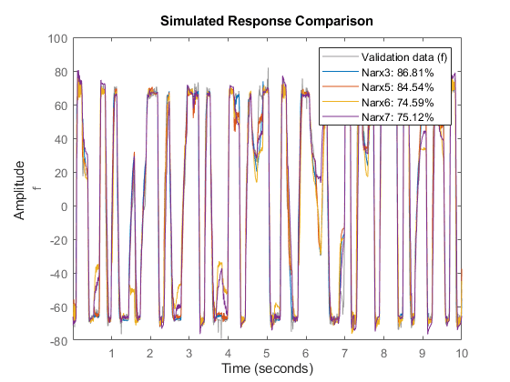
compare(zv, Narx3, Narx5, Narx6, Narx7) % comparison to validation data
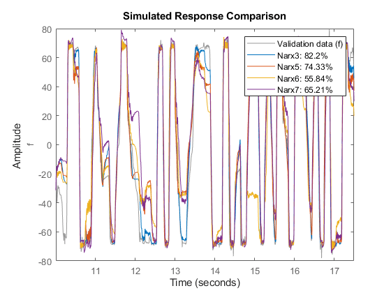
The models Narx6 and Narx7 seem to perform worse than Narx5, although we have not explored all the options associated with their estimation (such as choice of nonlinear regressors, number of units and other model orders).
Analyzing Estimated IDNLARX Models
Once a model has been identified and validated using the compare command, we may tentatively select the one that provides the best results without adding too much extra complexity. The selected model may then be analyzed further using commands such as plot and resid.
To get some insight into the nature of the nonlinearities of the model, inspect cross-sections of the nonlinear function F() in the estimated model f(t) = F(f(t-1), f(t-2), v(t-1),...,v(t-4)). For example, in model Narx5, the function F() is a sigmoid network. To explore the shape of the output of F() as a function of the regressors, use the plot command on the model:
plot(Narx5)
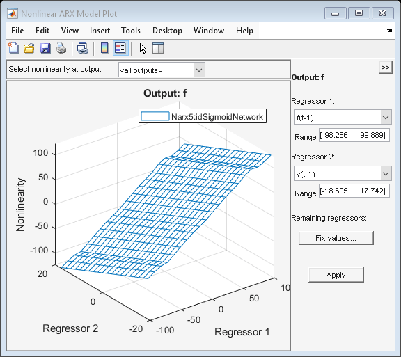
The plot window offers tools for selecting the cross-section regressors and their ranges. For more information, see "help idnlarx/plot".
The residual test can be used to further inspect the model. This test reveals if the prediction errors are white and uncorrelated to the input data.
set(gcf,'DefaultAxesTitleFontSizeMultiplier',1,...
   'DefaultAxesTitleFontWeight','normal',...
   'Position',[100 100 780 520]);
resid(zv, Narx3, Narx5)
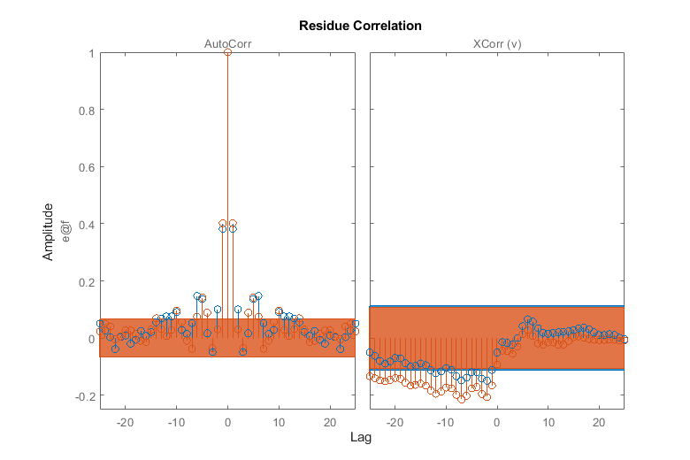
A failure of residual test may point to dynamics not captured by the model. For the model, Narx3, the residuals appear to be mostly within the 99% confidence bounds.
Creating Hammerstein-Wiener Models
The previously estimated nonlinear models are all of Nonlinear ARX (IDNLARX) type. Let us now try Hammerstein-Wiener (IDNLHW) models. These models represent a series connection of static nonlinear elements with a linear model. We may think of them as extensions of a linear output-error (OE) models wherein we subject the input and output signals of the linear model to static nonlinearities such as saturation or dead-zones.
Estimating an IDNLHW Model of Same Order as the Linear OE Model
The linear OE model LinMod2 was estimated using orders nb = 4, nf = 2 and nk = 1. Let us use the same orders for estimation of an IDNLHW model. We will use sigmoid network as nonlinearity for both input and output nonlinearities. The estimation is facilitated by the nlhw command. It is analogous to the oe command used for linear OE model estimation. However, in addition to model orders, we must also specify the names of, or objects for, the I/O nonlinearities.
Opt = nlhwOptions('SearchMethod','lm');
UNL = idSigmoidNetwork;
YNL = idSigmoidNetwork;
Nhw1 = nlhw(ze, [4 2 1], UNL, YNL, Opt)
Nhw1 =

<strong>Hammerstein-Wiener model with 1 output and 1 input</strong>

Linear transfer function corresponding to the orders nb = 4, nf = 2, nk = 1

Input nonlinearity: Sigmoid network with 10 units
Output nonlinearity: Sigmoid network with 10 units
Sample time: 0.005 seconds

Status:
Estimated using NLHW on time domain data "MR damper".
Fit to estimation data: 83.98%
FPE: 94.66, MSE: 88.34
Compare the response of this model against estimation and validation data sets:
clf
compare(ze, Nhw1); % comparison to estimation data
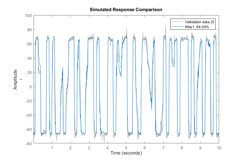
compare(zv, Nhw1); % comparison to validation data
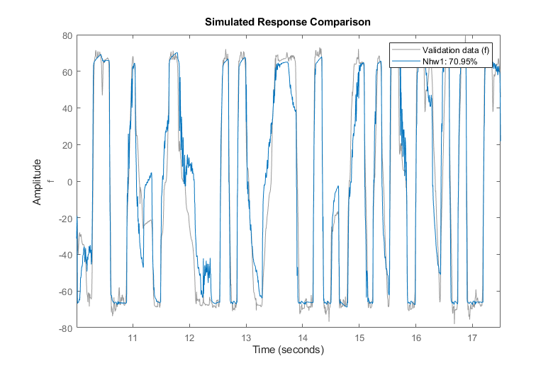
We observe about 70% fit to validation data using model Nhw1.
Analyzing Estimated IDNLHW Model
As for Nonlinear ARX models, the Hammerstein-Wiener models may be inspected for their nature of the I/O nonlinearities and the behavior of the linear component using the PLOT command. For more information, type "help idnlhw/plot" in MATLAB® Command Window.
plot(Nhw1)
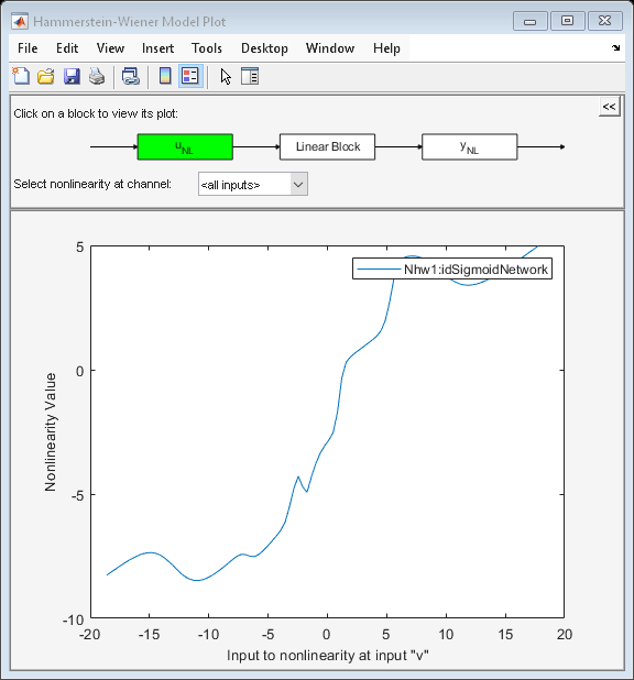
By default the input nonlinearity is plotted, showing that it may be simply a saturation function.
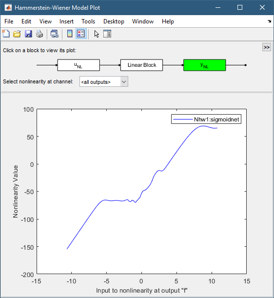
By clicking on the Y_NL icon, the output nonlinearity looks like a piecewise linear function.
Click on the Linear Block icon and choose Pole-Zero Map in the pull-down menu, it is then observed that a zero and a pole are quite close to each other, indicating that they may be removed, thereby reducing the model orders.
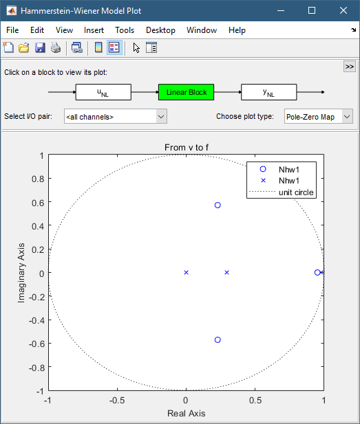
We will use this information to configure the structure of the model as shown next.
Trying Various Nonlinear Functions and Model Orders
Use saturation for input nonlinearity and sigmoid network for output nonlinearity, keeping the order of the linear component unchanged:
Nhw2 = nlhw(ze, [4 2 1], idSaturation, idSigmoidNetwork, Opt);
Use piecewise-linear nonlinearity for output and sigmoid network for input:
Nhw3 = nlhw(ze, [4 2 1], idSigmoidNetwork, idPiecewiseLinear, Opt);
Use a lower order linear model:
Nhw4 = nlhw(ze, [3 1 1], idSigmoidNetwork, idPiecewiseLinear, Opt);
We may also choose to "remove" nonlinearity at the input, output or both. For example, in order to use only an input nonlinearity (such models are called Hammerstein models), we may specify [] as output nonlinearity:
Nhw5 = nlhw(ze, [3 1 1],idSigmoidNetwork, [], Opt);
Compare all models
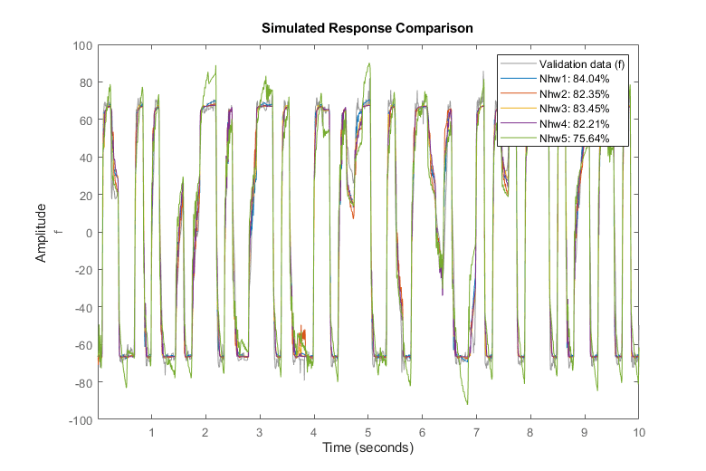
compare(ze, Nhw1, Nhw2, Nhw3, Nhw4, Nhw5) % comparison to estimation data
compare(zv, Nhw1, Nhw2, Nhw3, Nhw4, Nhw5) % comparison to validation data
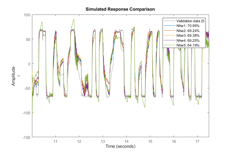
Nhw1 remains the best among all models, as shown by the comparison to validation data, but the other models, except Nhw5, have similar performance.
Conclusions
We explored various nonlinear models for describing the relationship between the voltage input and the damping force output. It was seen that among the Nonlinear ARX models, Narx2{6}, and Narx5 performed the best, while the model Nhw1 was the best among the Hammerstein-Wiener models. We also found that the Nonlinear ARX models provided the best option (best fits) for describing the dynamics of the MR damper.
Narx5.Name = 'Narx5';
Nhw1.Name = 'Nhw1';
compare(zv, LinMod2, Narx2{6}, Narx5, Nhw1)
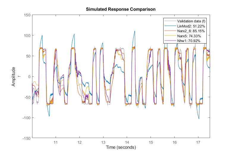
We found that there are multiple options available with each model type to fine-tune the quality of results. For Nonlinear ARX models, we can not only specify the model orders and the type of nonlinear functions, but also configure how the regressors are used and tweak the properties of the chosen functions. For Hammerstein-Wiener models, we can choose the type of input and output nonlinear functions, as well as the order of the linear component. For both model types, we have many choices of nonlinear functions available at our disposal to try and use. In lack of a particular preference for model structure or knowledge of the underlying dynamics, it is recommended to try the various choices and analyze their effect on the quality of the resulting models.
