Online State Estimation Using Identified Models - Linear Models

This example uses:

This example describes how to generate the state-transition and measurement functions for online state and output estimation using linear identification techniques.

System Identification Toolbox™ provides several recursive algorithms for state estimation such as Kalman Filter, Extended Kalman Filter (EKF), Unscented Kalman Filter (UKF), and Particle Filter (PF). Use of a state estimator requires specification of state and measurement dynamics:

How the system advances the states, represented by the state-transition equation $X (k + 1) = f (X (k), \dots)$ , where $X (k)$ is the state value at the time step $k$ ; the function $f (\cdot)$ can accept additional input arguments to accommodate any dependency on exogenous inputs and the time instant.
How the system computes the output or measurement $y (k)$ as a function of $X (k)$ and possibly some additional inputs; $y (k) = g (X (k), \dots)$

In addition, you are required to provide the covariance values of the various disturbances affecting the state and measurement dynamics. All filters execute a sequence of state value prediction (using $f (\cdot)$ ) and a correction of that prediction (using $g (\cdot)$ ) alternately. You have the option of performing multiple prediction steps before using the latest measurements to apply a correction.

This example shows how you can generate the required state-transition and measurement equations by using linear (black-box or grey-box) identification techniques. When identifying a linear model, the information regarding both the measurement dynamics (that is, how the output is related to the measured inputs) as well as the noise dynamics (that is, how the unmeasured disturbances influence the output) can be often be generated simultaneously. This results in a model of general structure:

$y (t) = G (q) u (t) + H (q) e (t)$

where $G (q)$ is called the measurement transfer function and $H (q)$ is called the noise transfer function. If the noise dynamics are not explicitly modeled, such as when using Output-Error (OE) model structure which results in a model of the form $y (t) = G (q) u (t) + e (t)$ , it is also often possible to extend the measurement model to account for the noise dynamics as a post-estimation model processing step.

Example System: An Industrial Robot Arm

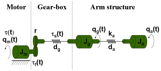
Consider a robot arm is described by a nonlinear three-mass flexible model. The input to the robot is the applied torque $u (t) = τ (t)$ generated by the electrical motor, and the resulting angular velocity of the motor $y (t) = \frac{d}{d t} q_{m} (t)$ is the measured output.

It is possible to derive the equations of motion for this system. For example, a nonlinear state-space description of this system that uses 5 states is described in the example titled "Modeling an Industrial Robot Arm".

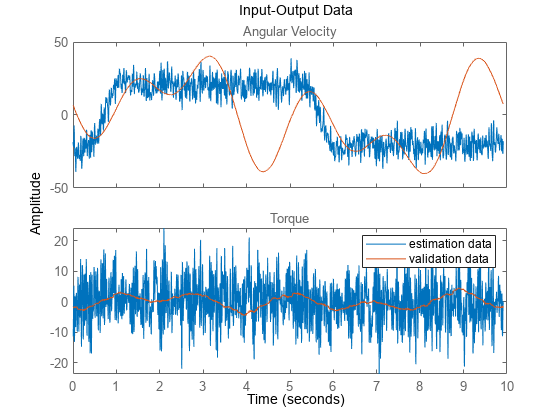
This system is excited with inputs of different profiles and the resulting angular velocity of the motor is recorded. A periodic excitation signal of approximately 10 seconds duration was employed to generate a reference speed for the controller. The chosen sampling frequency was 2 kHz (sample time Ts = 0.0005 seconds). For estimation (training) data, a multisine input signal with a flat amplitude spectrum in the frequency interval of 1-40 Hz with a peak value of 16 rad/s was used. The multisine signal is superimposed on a filtered square wave with amplitude 20 rad/s and cut-off frequency 1 Hz. For validation data, a multisine input signal containing frequencies 0.1, 0.3, and 0.5 Hz was used, with peak value of 40 rad/s.

Both datasets are downsampled 10 times for the purposes of the current example.

load robotarmdata.mat
% Prepare estimation data
eData = iddata(ye,ue,5e-4,'InputName','Torque','OutputName','Angular Velocity','Tstart',0);
eData = idresamp(eData,[1 10]);
eData.Name = 'estimation data';
% Prepare validation data
vData = iddata(yv3,uv3,5e-4,'InputName','Torque','OutputName','Angular Velocity','Tstart',0);
vData = idresamp(vData,[1 10]);
vData.Name = 'validation data';
idplot(eData, vData)
legend show

Black-Box LTI Models of System Dynamics

Suppose the equations of motion are not known. Then a dynamic model of the system can be derived by using a black-box identification approach such as using the ssest command (linear case) or the nlarx command (nonlinear case). In this first modeling attempt, make the assumption that the dynamics can be captured by a linear model. Use a linear model structure with a non-trivial noise component.

Black-Box State Space Model Identification

Identify a continuous-time state-space model of the best order in the 1:10 order range. This can be accomplished by running the following command which requires interactive selection of an order value from the model order selection dialog.

% linsys1 = ssest(eData, 1:10)  % uncomment to execute

The plot launched by running this command is:

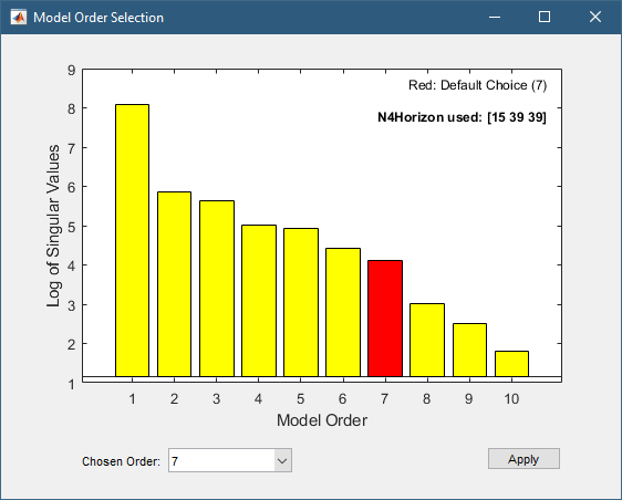
An order of 7 is suggested. The results obtained by selecting this value is equivalent to running the following commands:

% Set estimation options
opt = ssestOptions;
opt.N4Horizon = [15 39 39];
Order = 7;
% Run ssest to identify the model of chosen order and options
linsys1 = ssest(eData, Order, opt)

linsys1 =
  Continuous-time identified state-space model:
      dx/dt = A x(t) + B u(t) + K e(t)
       y(t) = C x(t) + D u(t) + e(t)
 
  A = 
           x1      x2      x3      x4      x5      x6      x7
   x1  -10.23  -34.14   9.669  -3.467   4.134   22.53  -6.348
   x2   2.111  -61.48  -133.3  -124.3   18.54   2.223   69.06
   x3    20.5   189.9  -16.59  -35.33   13.29  -25.67   16.48
   x4  -16.36    86.7    78.9  -11.04   84.22  -31.36   113.8
   x5   -1.54   16.24  -17.36  -80.65  -24.82   41.52  -71.55
   x6  -26.95  -108.9   79.27   70.97   32.15  -49.01   555.9
   x7    1.59   3.371   12.31  -22.04  -22.46   7.566  -132.4
 
  B = 
        Torque
   x1  -0.1109
   x2  -0.1055
   x3  0.07218
   x4  -0.1894
   x5   0.1187
   x6  -0.9121
   x7   0.2937
 
  C = 
                     x1      x2      x3      x4      x5      x6      x7
   Angular Velo    -852   45.74  -28.32  -22.72  -11.58   8.592  -1.034
 
  D = 
                 Torque
   Angular Velo       0
 
  K = 
       Angular Velo
   x1        -2.993
   x2         -2.95
   x3         16.37
   x4        -15.28
   x5        -3.674
   x6         2.207
   x7        -12.88
 
Parameterization:
   FREE form (all coefficients in A, B, C free).
   Feedthrough: none
   Disturbance component: estimate
   Number of free coefficients: 70
   Use "idssdata", "getpvec", "getcov" for parameters and their uncertainties.

Status:                                                     
Estimated using SSEST on time domain data "estimation data".
Fit to estimation data: 94.22% (prediction focus)           
FPE: 1.481, MSE: 1.45                                       
 
Model Properties

% Validate the model by checking how well it simulates the measured output in the validation dataset
compare(vData,linsys1)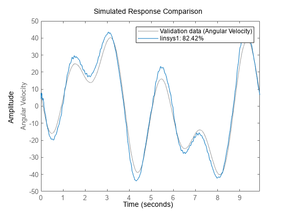

linsys1 is a 7th order continuous-time state-space model of the following structure:

$\begin{array}{l} \frac{dx (t)}{dt} = A x (t) + B u (t) + K e (t) \\ y (t) = C x (t) + e (t) \end{array}$

Here $e (t)$ are the output prediction errors. Note that the states most likely have no clear physical interpretation and the disturbance term $K e (t)$ cannot be treated as true process noise. However, for online output prediction, this model provides all the information needed. The state prediction by itself may not be of practical value since the states $x (t)$ are arbitrary. But the predicted states can be used to predict the output values using $y_{predicted} (t) = C x_{predicted} (t)$

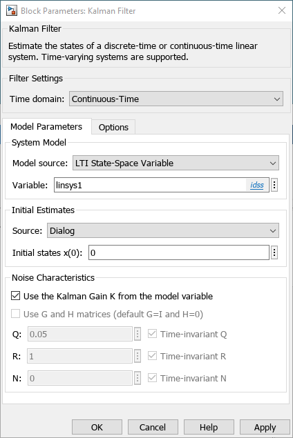
Configuring the Kalman Filter Block

Set Time domain drop-down selection to "Continuous-Time"
Set Model source to LTI State-Space Variable
Set Variable to linsys1
Under Noise Characteristics section, check the checkbox for "Use the Kalman Gain K from the model variable"

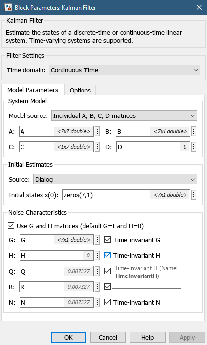
Alternatively, extract the system matrices, and the noise variances and specify them directly. For example, let $w (t)$ be a scalar disturbance source. Then another equivalent filter representation can be as follows:

[A,B,C,D,K] = idssdata(linsys1);
NV = linsys1.NoiseVariance;
G = K;
H = 0;
Q = NV;
R = NV;
N = NV;
% Verify using KALMAN command (requires Control System Toolbox)
% (Estimated Kalman Gain Kest is same as the identified K matrix)
[~,Kest] = kalman(ss(A,[B, G],C,[D H]),Q,R,N)

Kest = 7×1

   -2.9928
   -2.9504
   16.3689
  -15.2789
   -3.6738
    2.2074
  -12.8844

Note that the Kalman Filter block supports both continuous and discrete-time models.

Configuring the Extended Kalman Filter (EKF) Block

While not required for linear systems, you can also implement the state estimator as an Extended Kalman Filter (EKF). To do so, you need a discrete-time model. You can use c2d to discretize the previously identified linsys1. Alternatively, you can directly identify a discrete-time model using the ssest command.

opt = ssestOptions;
opt.N4Horizon = [15 39 39];
Order = 7;
% Identify a discrete-time state space model
linsys2 = ssest(eData, Order, opt, 'Ts', eData.Ts)

linsys2 =
  Discrete-time identified state-space model:
    x(t+Ts) = A x(t) + B u(t) + K e(t)
       y(t) = C x(t) + D u(t) + e(t)
 
  A = 
              x1         x2         x3         x4         x5         x6         x7
   x1     0.9611    -0.1484    0.05979    0.01731    0.03113   -0.05424  -0.002952
   x2    -0.0283     0.3138    -0.5373    -0.4152   -0.03035    -0.1583     0.1633
   x3     0.1075     0.6587     0.5894    -0.3731   -0.01745    0.06084     0.1164
   x4   -0.05058     0.4633      0.122     0.6973     0.3778    -0.1713     0.2899
   x5    0.01611    -0.1049   -0.07019    -0.3398     0.8932      0.178    -0.2024
   x6    -0.1259     -0.177     0.4843     0.1126     0.1429     0.3777      1.714
   x7   -0.02454    0.04994     0.0622    -0.1431   -0.09169   -0.01395    0.08604
 
  B = 
          Torque
   x1   -0.00127
   x2  -0.002701
   x3   0.003675
   x4  -0.002421
   x5   0.001166
   x6  -0.002035
   x7   0.002307
 
  C = 
                      x1       x2       x3       x4       x5       x6       x7
   Angular Velo   -851.7    43.61   -28.55   -24.43   -9.701   0.5012  0.05347
 
  D = 
                 Torque
   Angular Velo       0
 
  K = 
       Angular Velo
   x1     -0.002365
   x2      0.003396
   x3       0.01062
   x4     -0.001163
   x5      0.005198
   x6      0.006216
   x7     -0.004374
 
Sample time: 0.005 seconds

Parameterization:
   FREE form (all coefficients in A, B, C free).
   Feedthrough: none
   Disturbance component: estimate
   Number of free coefficients: 70
   Use "idssdata", "getpvec", "getcov" for parameters and their uncertainties.

Status:                                                     
Estimated using SSEST on time domain data "estimation data".
Fit to estimation data: 97.08% (prediction focus)           
FPE: 0.38, MSE: 0.3694                                      
 
Model Properties

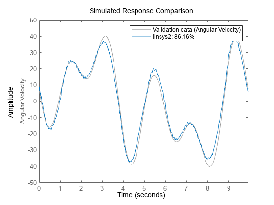
compare(vData,linsys2)

The EKF block requires the state transition and the measurement functions to be specified as MATLAB functions.

% Prepare data
% Extract system matrices in order to define the state-transition and measurement functions
[Ad,Bd,Cd,Dd,Kd] = idssdata(linsys2);
NVd = linsys2.NoiseVariance; % measurement noise variance
StateNoiseCovariance_d = Kd*NV*Kd';
Ts = linsys2.Ts;

The state transition function is simply $x (t + 1) = A_{d} x (t) + B_{d} u (t_{)})$ , while the measurement function is $y (t) = C_{d} x (t) + D_{d} u (t)$ . These are implemented using the Simulink Function blocks called stateTransitionFcn and measurementFcn, respectively, in the Simulink model StateEstimation_Using_LinearModel.slx.

open_system('StateEstimation_Using_LinearModel')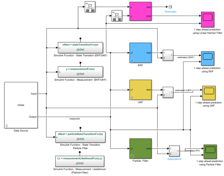

Configuring the Unscented Kalman Filter (UKF) Block

The UKF block is configured in an identical manner as the EKF block. In the stateEstimation_Using_LinearModel model, the Simulink functions called stateTransitionFcn and measurementFcn are shared by both the EKF and UKF blocks.

Configuring the Particle Filter Block

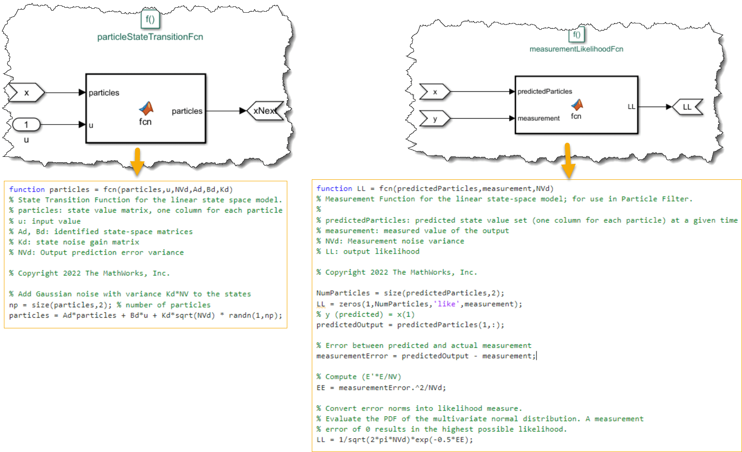
It is similarly possible to use the linear state-space equations to perform state estimation using the Particle Filter. For this example, you use 1000 particles and assume a Gaussian distribution of the state and measurement errors. See the Simulink functions particleStateTransitionFcn and measurementLikelihoodFcn for how the particles are moved and the output likelihood computed.

NumParticles = 1000;

Online State Estimation Performance

Compare the performance of the Kalman filter, Extended Kalman Filter (EKF), Unscented Kalman Filter (UKF), and Particle Filter (PF) for 1-step, and 10-step ahead state/output predictions.

1-Step Prediction Results

The quality of the state estimation can be judged by how well the estimated states reconstruct the measured output.

sim('StateEstimation_Using_LinearModel');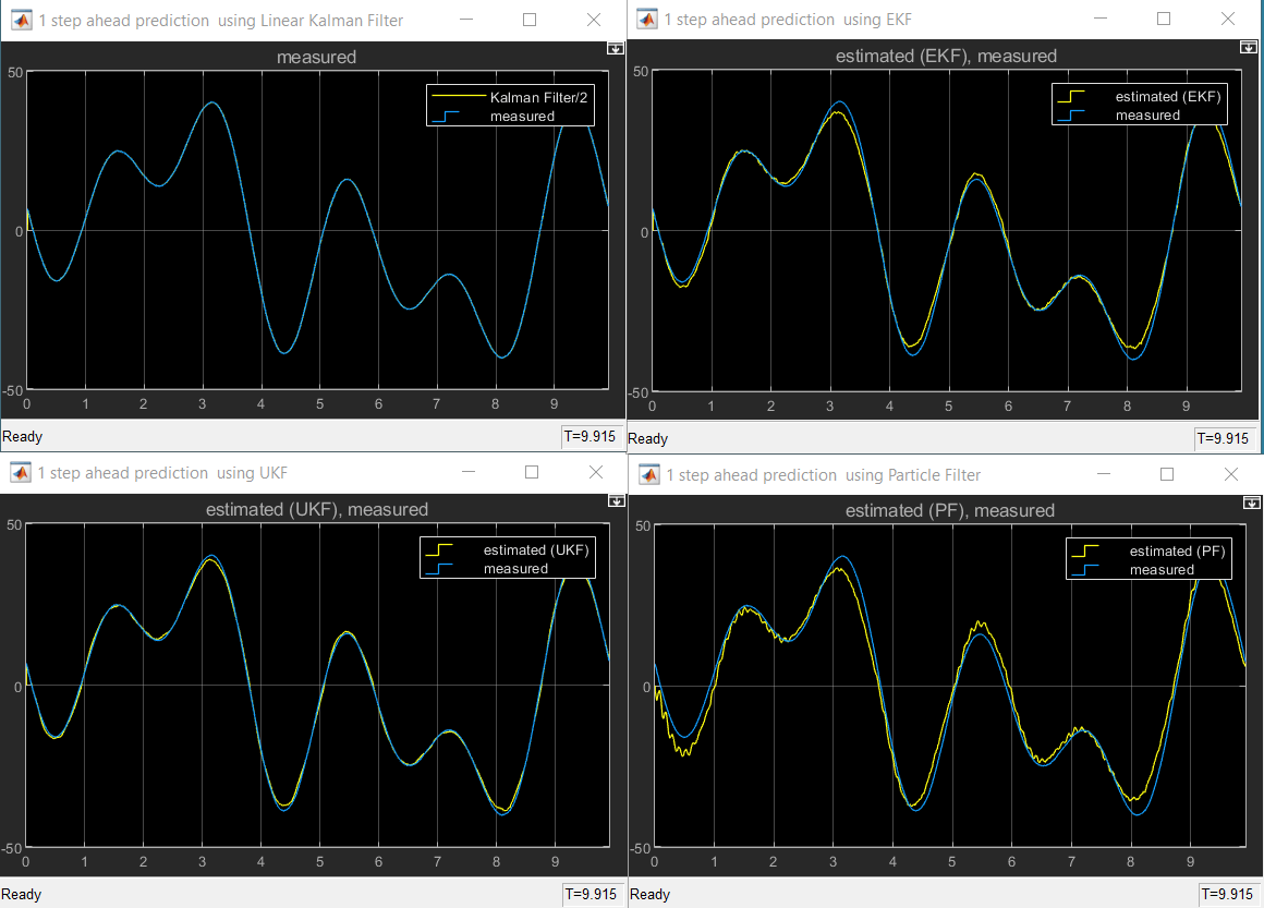

The scopes show the comparison of the measured output against the predicted one. The continuous-time, linear, Kalman filter provides the best fit; the other (nonlinear) estimators also show good fits. However, the estimation is performed only one step ahead, which is typically more accurate than longer horizon predictions, where the measurements are used at a smaller frequency to update the predictions. Doing predictions and corrections at different rates requires enabling the multi-rate technique in the filter blocks.

Multi-Rate Technique for Longer Horizon Prediction

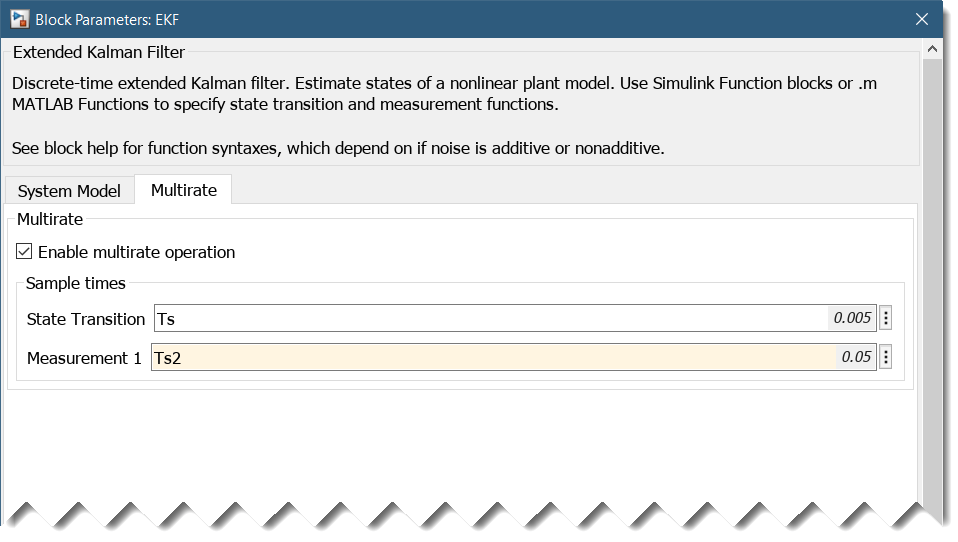
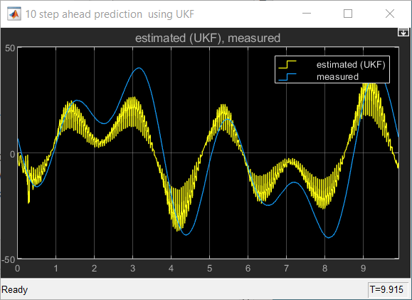
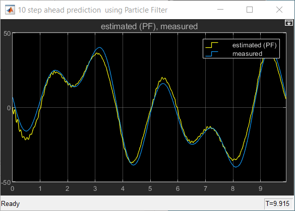
Multi-rate operation is supported for the nonlinear state estimators - EKF, UKF and Particle filters. Choose to correct the predictions using measurements once for every 10 predictions. This effectively achieves a 10-step ahead prediction.

Ts2 = 10*Ts; % correction interval (Ts is prediction interval)

Enable multi-rate operation under the corresponding tab of the filter dialog.

In order to provide the measurements at a slower rate, you also need to insert rate transition blocks at the input ports of the EKF, UKF, and Particle Filter blocks. This is implemented in the model StateEstimation_Using_LinearModelMultiRate.slx.

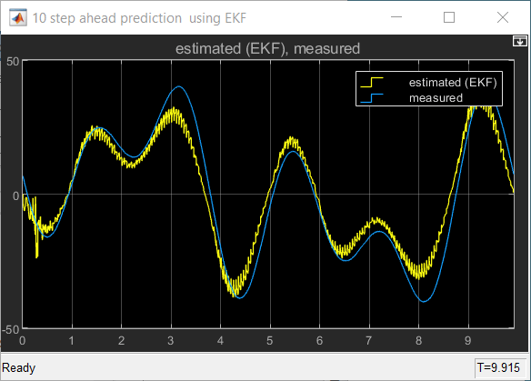
open_system('StateEstimation_Using_LinearModelMultiRate')
sim('StateEstimation_Using_LinearModelMultiRate');

10-Step Prediction Results

The filter performance is not as good as in the 1-step ahead prediction case where you are able to correct the predictions at each time instant. The longer-term predictions can be improved by using nonlinear models.

Linear Time Invariant Box-Jenkins (BJ) Polynomial Model

The linear model chosen to provide the measured and noise dynamics need not be based on a state-space form. You can identify a model of any structure, although it is preferable to use a form that contains a nontrivial noise component (that is, $H (q) \neq 1$ ). With such models, the state predictors have the ability to perform corrections using available measurements in real-time applications.

As an example, estimate a Box-Jenkins polynomial model and convert it into a state-space form.

% Estimate a Box-Jenkins model of orders nb=nf=5, nc=nd=3, nk=1
sysBJ = bj(eData,[5 3 3 5 1])

sysBJ =
Discrete-time BJ model: y(t) = [B(z)/F(z)]u(t) + [C(z)/D(z)]e(t)             
  B(z) = 0.8549 z^-1 - 1.104 z^-2 + 0.4614 z^-3 + 0.3785 z^-4 - 0.5058 z^-5  
                                                                             
  C(z) = 1 + 0.9427 z^-1 + 0.818 z^-2 + 0.2944 z^-3                          
                                                                             
  D(z) = 1 - 1.404 z^-1 + 1.054 z^-2 - 0.5757 z^-3                           
                                                                             
  F(z) = 1 - 1.781 z^-1 + 1.009 z^-2 + 0.3544 z^-3 - 0.987 z^-4 + 0.4076 z^-5
                                                                             
Sample time: 0.005 seconds
  
Parameterization:
   Polynomial orders:   nb=5   nc=3   nd=3   nf=5   nk=1
   Number of free coefficients: 16
   Use "polydata", "getpvec", "getcov" for parameters and their uncertainties.

Status:                                                  
Estimated using BJ on time domain data "estimation data".
Fit to estimation data: 95.73% (prediction focus)        
FPE: 0.8102, MSE: 0.7909                                 
 
Model Properties

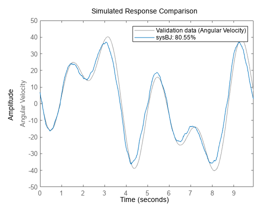
% Validate the model
compare(vData, sysBJ)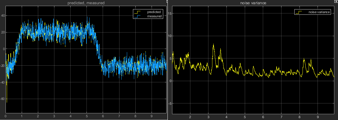

% Convert the model into state-space form
sysSS = idss(sysBJ)

sysSS =
  Discrete-time identified state-space model:
    x(t+Ts) = A x(t) + B u(t) + K e(t)
       y(t) = C x(t) + D u(t) + e(t)
 
  A = 
            x1       x2       x3       x4       x5       x6       x7       x8
   x1    1.781   -1.009  -0.3544    0.987  -0.8153        0        0        0
   x2        1        0        0        0        0        0        0        0
   x3        0        1        0        0        0        0        0        0
   x4        0        0        1        0        0        0        0        0
   x5        0        0        0      0.5        0        0        0        0
   x6        0        0        0        0        0    1.404   -1.054   0.5757
   x7        0        0        0        0        0        1        0        0
   x8        0        0        0        0        0        0        1        0
 
  B = 
       Torque
   x1       2
   x2       0
   x3       0
   x4       0
   x5       0
   x6       0
   x7       0
   x8       0
 
  C = 
                      x1       x2       x3       x4       x5       x6       x7       x8
   Angular Velo   0.4275  -0.5519   0.2307   0.1893  -0.5058    1.173  -0.1179   0.4351
 
  D = 
                 Torque
   Angular Velo       0
 
  K = 
       Angular Velo
   x1             0
   x2             0
   x3             0
   x4             0
   x5             0
   x6             2
   x7             0
   x8             0
 
Sample time: 0.005 seconds

Parameterization:
   FREE form (all coefficients in A, B, C free).
   Feedthrough: none
   Disturbance component: estimate
   Number of free coefficients: 88
   Use "idssdata", "getpvec", "getcov" for parameters and their uncertainties.

Status:                                 
Created by conversion from idpoly model.
 
Model Properties

sysSS is a state-space model that can be used in various types of filters as discussed above.

Grey-Box LTI Models

A structured or a grey-box modeling approach is used when the governing equations of motion are known, but the values of one or more coefficients used in these equations need to be estimated. A generic linear representation of a stochastic state-space model is:

$\begin{array}{l} \dot{x} = Ax (t) + Bu (t) + Gw (t) \\ y (t) = Cx (t) + Du (t) + Hw (t) + v (t) \end{array}$

where $w (t)$ denotes process noise and $v (t)$ represents output measurement noise; both are white noise processes. For the purpose of this example, suppose the ideal governing equations in a noise-free form are known. For example, this could be a set of differential or difference equations relating $y (t)$ to $u (t)$ . In a state-space representation, this means that A, B, C, D matrices are known, However, the effect of noise properties can be harder to determine and require separate experimentation.

A linear approximation of the robot arm dynamics is as follows:

$\begin{array}{l} State definition : \\ x_{1} (t) = q_{m} (t) - q_{g} (t) \\ x_{2} (t) = q_{g} (t) - q_{a} (t) \\ x_{3} (t) = {\dot{q}}_{m} (t) \\ x_{4} (t) = {\dot{q}}_{g} (t) \\ x_{5} (t) = {\dot{q}}_{a} (t) \end{array}$

$\begin{array}{l} Linearized equations of motion : \\ {\dot{x}}_{1} (t) = x_{3} (t) - x_{4} (t) \\ {\dot{x}}_{2} (t) = x_{4} (t) - x_{5} (t) \\ {\dot{x}}_{3} (t) = - k_{31} x_{1} - k_{33} x_{3} + k_{34} x_{4} + bu (t) \\ {\dot{x}}_{4} (t) = k_{41} x_{1} - k_{42} x_{2} + k_{43} x_{3} - k_{44} x_{4} + k_{45} x_{5} \\ {\dot{x}}_{5} (t) = k_{52} x_{2} + k_{5} (x_{4} (t) - x_{5} (t)) \\ y (t) = x_{3} (t) \end{array}$

The tunable parameters are $k_{31}, k_{33}, k_{34}, b, k_{41}, k_{42}, k_{43}, k_{44}, k_{45}, k_{52}, k_{5}$ with the constraint that all are non-negative. In state-space form, these equations can be written as:

$A = (\begin{array}{c} 0 & 0 & 1 & - 1 & 0 \\ 0 & 0 & 0 & 1 & - 1 \\ - k_{31} & 0 & - k_{33} & k_{34} & 0 \\ k_{41} & - k_{42} & k_{43} & - k_{44} & k_{45} \\ 0 & k_{52} & 0 & k_{5} & - k_{5} \end{array})$ , $B = (\begin{array}{c} 0 \\ 0 \\ b \\ 0 \\ 0 \end{array})$ , $C = (\begin{array}{c} 0 & 0 & 1 & 0 & 0 \end{array}), D = 0$

The physical knowledge leading to these equations do not enlighten us about the nature of the process disturbances. Embed these equations into a stochastic form by adding process noise and measurement noise terms.

$\begin{array}{l} \dot{X} (t) = AX (t) + Bu (t) + w (t) \\ y (t) = CX (t) + Du (t) + v (t) \end{array}$

where $w (t)$ and $v (t)$ are independent white-noise terms with covariance matrices $R_{w} = E {{ww}^{'}}, R_{y} = E {{vv}^{'}}$ . Assume that $R_{w}$ to be a diagonal matrix with unknown entries. Also assume that $R_{y}$ is known to be equal to 1.

In this form, the unknowns to be estimated are: $k_{31}, k_{33}, k_{34}, b, k_{41}, k_{42}, k_{43}, k_{44}, k_{45}, k_{52}, k_{5}, r_{w1}, r_{w2}, r_{w3}, r_{w4}, r_{w5}$ , where $r_{wi}, i = 1, . ., 5$ are the diagonal entries of $R_{w} .$ In order to estimate these values, use the linear grey-box modeling framework. This typically involves 4 steps.

Step 1: Prepare the ODE Function

Write a MATLAB function (called an ODE file) that computes the state-space matrices (in the innovations form) as a function of these unknowns.

type robotARMLinearODE

function [A,B,C,D,K] = robotARMLinearODE(k31,k33,k34,b,k41,k42,k43,k44,k45,k52,k5,r,Ts,varargin)
% Linear ODE file for use in linear grey box model identification.
% k*: unknown coefficients of the A matrix
% b: unknown coefficient in the B matrix
% r*: unknown entries of the process noise covariance matrix

% Copyright 2022 The MathWorks, Inc.

Warn = warning('off','Ident:estimation:PredictorCorrectionFailure');
warning off 'Control:design:MustBePositiveDefinite'
Clean = onCleanup(@()warning(Warn));
A = [ 0,    0,   1,   -1,   0; 
      0,    0,   0,    1,  -1; 
     -k31,  0,  -k33,  k34, 0;
      k41, -k42, k43, -k44, k45;
      0,    k52, 0,    k5, -k5];

B = [0,0,b,0,0]';
C = [0,0,1,0,0];
D = 0;
Rw = diag(r);
Ry = 1;
% Compute Kalman gain (requires Control System Toolbox)
if norm(r,inf)<1e-12
   K = zeros(5,1);
else
   [~,K] = kalman(ss(A,eye(5),C,0,0),Rw,Ry); 
end

Step 2: Create a Linear Grey Box Template Model (idgrey object)

Create a template idgrey model that puts together the ODE function and the initial guess values of its parameters.

% Specify the name or function handle to the MATLAB function that specifies the ODE equations
ODEFun = @robotARMLinearODE;

% Assign initial guess values to the model's parameters
Fv = 0.00986347;
J = 0.032917;
a_m = 0.17911;
a_g = 0.612062;
k_g = 20.5927;
d_g = 0.0624181;
k_a =  20.2307;
d_a = 0.00987528;

b = 1/J/a_m;
k31 = b*k_g;
k33 = b*(d_g+Fv);
k34 = b*d_g;
k41 = 1/J/a_g*k_g;
k42 = 1/J/a_g*k_a;
k43 = 1/J/a_g*d_g;
k44 = 1/J/a_g*(d_g+d_a);
k45 = 1/J/a_g*d_a;
k52 = k_a/J/(1-a_m-a_g);
k5 = d_a/J/(1-a_m-a_g);

r = zeros(1,5); % diagonal entries of R_w
ParameterGuess = {'k31',k31;...
   'k33',k33; ...
   'k34',k34; ...
   'b',b; ...
   'k41',k41;...
   'k42',k42;...
   'k43',k43;...
   'k44',k44;...
   'k45',k45;
   'k52',k52;...
   'k5',k5;...
   'r',r};

% Create an idgrey model by assigning the ODE function and the initial guess values for all the
% parameters. Use 'c' to denote that the ODE function uses a continuous-time description.
sysGRini = idgrey(ODEFun,ParameterGuess,'c',[],0)

sysGRini =
  Continuous-time linear grey box model defined by @robotARMLinearODE function:
      dx/dt = A x(t) + B u(t) + K e(t)
       y(t) = C x(t) + D u(t) + e(t)
 
  A = 
           x1      x2      x3      x4      x5
   x1       0       0       1      -1       0
   x2       0       0       0       1      -1
   x3   -3493       0  -12.26   10.59       0
   x4    1022   -1004   3.098  -3.588  0.4902
   x5       0    2943       0   1.437  -1.437
 
  B = 
          u1
   x1      0
   x2      0
   x3  169.6
   x4      0
   x5      0
 
  C = 
       x1  x2  x3  x4  x5
   y1   0   0   1   0   0
 
  D = 
       u1
   y1   0
 
  K = 
       y1
   x1   0
   x2   0
   x3   0
   x4   0
   x5   0
 
  Model parameters:
   k31 = 3493
   k33 = 12.26
   k34 = 10.59
   b = 169.6
   k41 = 1022
   k42 = 1004
   k43 = 3.098
   k44 = 3.588
   k45 = 0.4902
   k52 = 2943
   k5 = 1.437
   r = 
    0    0    0    0    0
 
 
Parameterization:
   ODE Function: @robotARMLinearODE
   Disturbance component: parameterized by the ODE function
   Initial state: 'auto'
   Number of free coefficients: 16
   Use "getpvec", "getcov" for parameters and their uncertainties.

Status:                                                         
Created by direct construction or transformation. Not estimated.
 
Model Properties

% Lower bound the parameters (all parameters >=0)
P = sysGRini.Structure.Parameters;
for i = 1:numel(P)
   P(i).Minimum = 0;
end
sysGRini.Structure.Parameters = P;

Step 3: Estimate Model Parameters

Perform estimation using the greyest command.

opt = greyestOptions;
Wid = warning('off','Ident:estimation:PredictorCorrectionFailure');
WarnResetter = onCleanup(@()warning(Wid));
% Fix the initial states to zeros (they will not be updated by estimation)
opt.InitialState = zeros(5,1);
% Estimate model parameters
sysGR = greyest(eData, sysGRini, opt)

sysGR =
  Continuous-time linear grey box model defined by @robotARMLinearODE function:
      dx/dt = A x(t) + B u(t) + K e(t)
       y(t) = C x(t) + D u(t) + e(t)
 
  A = 
              x1         x2         x3         x4         x5
   x1          0          0          1         -1          0
   x2          0          0          0          1         -1
   x3      -2102          0     -7.171      9.767          0
   x4      721.2     -411.5    0.05869     -2.068  0.0008415
   x5          0       3886          0      17.25     -17.25
 
  B = 
       Torque
   x1       0
   x2       0
   x3   120.7
   x4       0
   x5       0
 
  C = 
                 x1  x2  x3  x4  x5
   Angular Velo   0   0   1   0   0
 
  D = 
                 Torque
   Angular Velo       0
 
  K = 
       Angular Velo
   x1        -1.263
   x2       -0.1483
   x3         65.71
   x4        -2.804
   x5         4.162
 
  Model parameters:
   k31 = 2102
   k33 = 7.171
   k34 = 9.767
   b = 120.7
   k41 = 721.2
   k42 = 411.5
   k43 = 0.05869
   k44 = 2.068
   k45 = 0.0008415
   k52 = 3886
   k5 = 17.25
   r = 
      3.96    0.1688      5.82     290.8      8755
 
 
Parameterization:
   ODE Function: @robotARMLinearODE
   Disturbance component: parameterized by the ODE function
   Initial state: fixed to double value
   Number of free coefficients: 16
   Use "getpvec", "getcov" for parameters and their uncertainties.

Status:                                                       
Estimated using GREYEST on time domain data "estimation data".
Fit to estimation data: 86.94% (prediction focus)             
FPE: 7.523, MSE: 7.403                                        
 
Model Properties

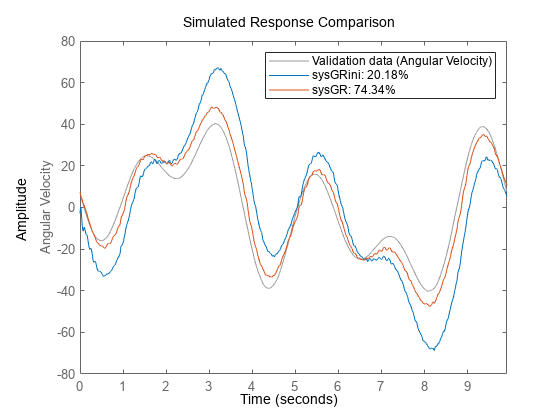
Step 4: Model Validation

compare(vData,sysGRini,sysGR)

Finally, convert the model into the standard linear-space form (idss), and/or extract state-space matrices from it for use in the various state estimators using the idssdata command.

sysSSgr = idss(sysGR)

sysSSgr =
  Continuous-time identified state-space model:
      dx/dt = A x(t) + B u(t) + K e(t)
       y(t) = C x(t) + D u(t) + e(t)
 
  A = 
              x1         x2         x3         x4         x5
   x1          0          0          1         -1          0
   x2          0          0          0          1         -1
   x3      -2102          0     -7.171      9.767          0
   x4      721.2     -411.5    0.05869     -2.068  0.0008415
   x5          0       3886          0      17.25     -17.25
 
  B = 
       Torque
   x1       0
   x2       0
   x3   120.7
   x4       0
   x5       0
 
  C = 
                 x1  x2  x3  x4  x5
   Angular Velo   0   0   1   0   0
 
  D = 
                 Torque
   Angular Velo       0
 
  K = 
       Angular Velo
   x1        -1.263
   x2       -0.1483
   x3         65.71
   x4        -2.804
   x5         4.162
 
Parameterization:
   STRUCTURED form (some fixed coefficients in  A, B, C).
   Feedthrough: none
   Disturbance component: estimate
   Number of free coefficients: 17
   Use "idssdata", "getpvec", "getcov" for parameters and their uncertainties.

Status:                                 
Created by conversion from idgrey model.
 
Model Properties

[A,B,C,D,K] = idssdata(sysGR);
NV = sysGR.NoiseVariance;

Linear Time-Varying Models

One of the important reasons for using Kalman filters is to perform accurate predictions when the system itself is changing over time. In the Kalman Filter block, time-varying estimation is enabled by feeding in the system matrices as signals (set the Model source drop-down option to "Input port" and press Apply in the block's parameters dialog).

However, offline estimation algorithms such as ssest cannot identify time-varying systems. To do so, you must use the recursive estimation blocks provided in the Estimators library of System Identification Toolbox block library (slident). In particular, use the Recursive Polynomial Model Estimator block to recursively estimate the coefficients of polynomial models of various structures such as ARX, Output-Error (OE) or Box-Jenkins (BJ). You can feed the parameter values computed by this block into a Model Type Converter block in order to obtain the state-space matrices required by the Kalman filter.

The ARMAX Recursive Estimator

For this example, use a recursive ARMAX estimator. Then compute the A, B, C, D matrices and process noise matrix G from the estimated parameters using the Model Type Converter blocks.

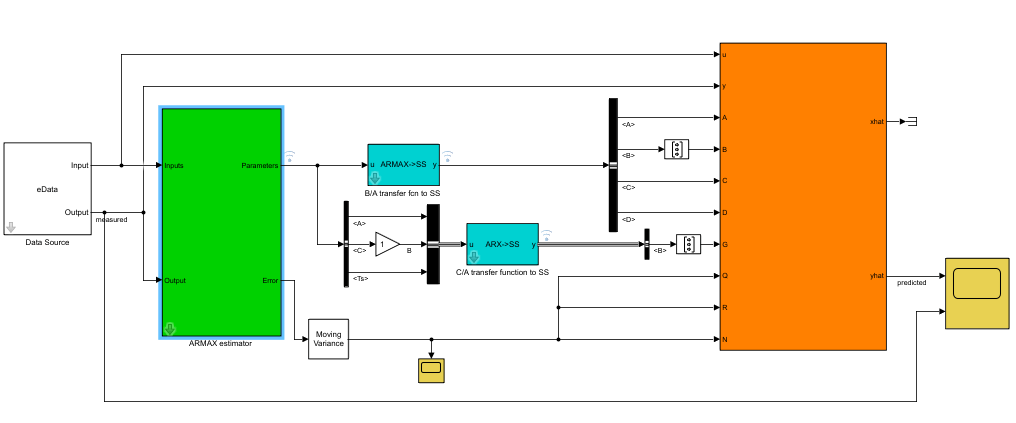
open_system('TimeVaryingStateEstimator')

The G matrix is computed by taking the A, C polynomial estimates from the ARMAX estimator, renaming bus signal C to B and then passing it to the Model Type Converter block. The rename is required since the Model Type Converter works only with measured dynamics of the polynomial model ( $B (q) / A (q)$ transfer function from the ARMAX model $A (q) y (t) = B (q) u (t) + C (q) e (t)$ ), but the dynamics we are interested in generating concerns the noise ( $C (q) / A (q)$ ) transfer function from the ARMAX model.

Estimation Results

Simulation of the model shows good tracking of the measured output.

sim('TimeVaryingStateEstimator');

The first plot (left) compares the measured output (blue) against the values predicted by the time varying Kalman filter (yellow). The second plot (right) shows the output error variance as estimated by the ARMAX estimator block. The computation is performed using the Moving Variance block from DSP System Toolbox™.