Regularized Identification of Dynamic Systems
This example shows the benefits of regularization for identification of linear and nonlinear models.
What Is Regularization
When a dynamic system is identified using measured data, the parameter estimates are determined as:
where the criterion typically is a weighted quadratic norm of the prediction errors . An regularized criterion is modified as:
A common special case of this is when . This is called ridge regression in statistics, e.g., see the ridge command in Statistics and Machine Learning Toolbox™.
A useful way of thinking about regularization is that represents prior knowledge about the unknown parameter vector and that describes the confidence in this knowledge. (The larger , the higher confidence). A formal interpretation in a Bayesian setting is that has a prior distribution that is Gaussian with mean and covariance matrix , where is the variance of the innovations.
The use of regularization can therefore be linked to some prior information about the system. This could be quite soft, like that the system is stable. The regularization variables and can be seen as tools to find a good model complexity for best tradeoff between bias and variance. The regularization constants and are represented by options called Lambda and R respectively in System Identification Toolbox™. The choice of is controlled by the Nominal regularization option.
Bias - Variance Tradeoff in FIR modeling
Consider the problem of estimating the impulse response of a linear system as an FIR model:
These are estimated by the command: m = arx(z,[0 nb 0]). The choice of order nb is a tradeoff between bias (large nb is required to capture slowly decaying impulse responses without too much error) and variance (large nb gives many parameters to estimate which gives large variance).
Let us illustrate it with a simulated example. We pick a simple second order Butterworth filter as system:
Its impulse response is shown in Figure 1:
trueSys = idtf([0.02008 0.04017 0.02008],[1 -1.561 0.6414],1);
[y0,t] = impulse(trueSys);
plot(t,y0)
xlabel('Time (seconds)'), ylabel('Amplitude'), title('Impulse Response')

Figure 1: The true impulse response.
The impulse response has decayed to zero after less than 50 samples. Let us estimate it from data generated by the system. We simulate the system with low-pass filtered white noise as input and add a small white noise output disturbance with variance 0.0025 to the output. 1000 samples are collected. This data is saved in the regularizationExampleData.mat file and shown in Figure 2.
load regularizationExampleData.mat eData
plot(eData)

Figure 2: The data used for estimation.
To determine a good value for nb we basically have to try a few values and by some validation procedure evaluate which is best. That can be done in several ways, but since we know the true system in this case, we can determine the theoretically best possible value, by trying out all models with nb=1,...,50 and find which one has the best fit to the true impulse response. Such a test shows that nb = 13 gives the best error norm (mse = 0.2522) to the impulse response. This estimated impulse response is shown together with the true one in Figure 3.
nb = 13;
m13 = arx(eData,[0 nb 0]);
[y13,~,~,y13sd] = impulse(m13,t);
plot(t,y0,t,y13)
xlabel('Time (seconds)'), ylabel('Amplitude'), title('Impulse Response')
legend('True system','13:th order FIR model')
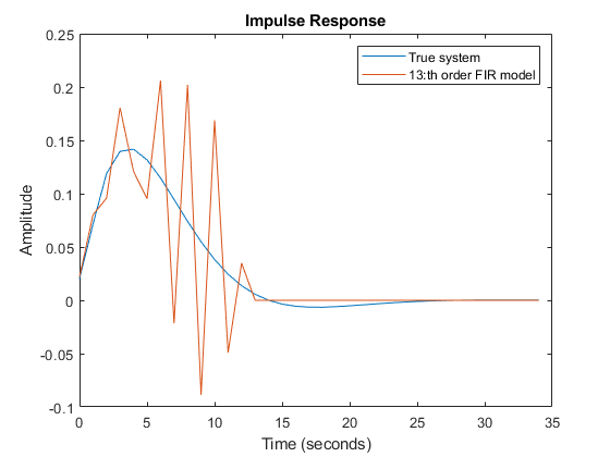
Figure 3: The true impulse response together with the estimate for order nb = 13.
Despite the 1000 data points with very good signal to noise ratio the estimate is not impressive. The uncertainty in the response is also quite large as shown by the 1 standard deviation values of response. The reason is that the low pass input has poor excitation.
plot(t,y0,t,y13,t,y13+y13sd,'r:',t,y13-y13sd,'r:')
xlabel('Time (seconds)'), ylabel('Amplitude'), title('Impulse Response')
legend('True system','13:th order FIR model','Bounds')
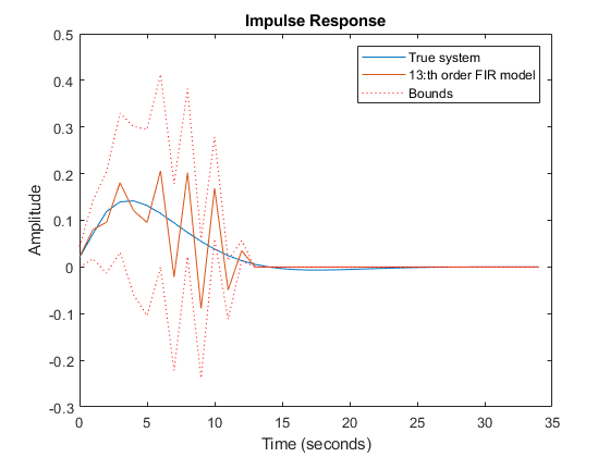
Figure 4: Estimated response with confidence bounds corresponding to 1 s.d.
Let us therefore try to reach a good bias-variance trade-off by ridge regression for a FIR model of order 50. Use arxOptions to configure the regularization constants. For this exercise we apply a simple penalty of .
aopt = arxOptions;
aopt.Regularization.Lambda = 1;
m50r = arx(eData, [0 50 0], aopt);
The resulting estimate has an error norm of 0.1171 to the true impulse response and is shown in Figure 5 along with the confidence bounds.
[y50r,~,~,y50rsd] = impulse(m50r,t);
plot(t,y0,t,y50r,t,y50r+y50rsd,'r:',t,y50r-y50rsd,'r:')
xlabel('Time (seconds)'), ylabel('Amplitude'), title('Impulse Response')
legend('True system','50:th order regularized estimate')
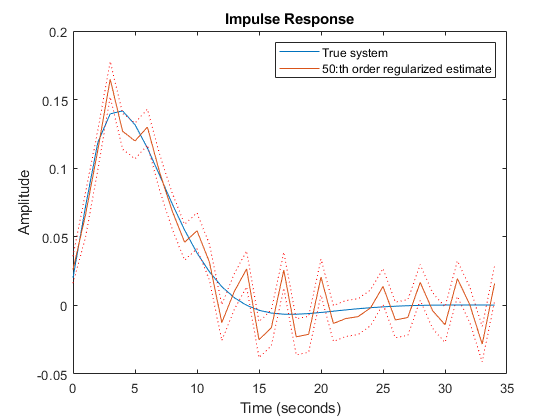
Figure 5: The true impulse response together with the ridge-regularized estimate for order nb = 50.
Clearly even this simple choice of regularization gives a much better bias-variance tradeoff, than selecting an optimal FIR order with no regularization.
Automatic Determination of Regularization Constants for FIR Models
We can do even better. By using the insight that the true impulse response decays to zero and is smooth, we can tailor the choice of to the data. This is achieved by the arxRegul function.
[L,R] = arxRegul(eData,[0 50 0],arxRegulOptions('RegularizationKernel','TC'));
aopt.Regularization.Lambda = L;
aopt.Regularization.R = R;
mrtc = arx(eData, [0 50 0], aopt);
[ytc,~,~,ytcsd] = impulse(mrtc,t);
arxRegul uses fmincon from Optimization Toolbox™ to compute the hyper-parameters associated with the regularization kernel ("TC" here). If Optimization Toolbox is not available, a simple Gauss-Newton search scheme is used instead; use the "Advanced.SearchMethod" option of arxRegulOptions to choose the search method explicitly. The estimated hyper-parameters are then used to derive the values of and .
Using the estimated values of and in ARX leads to an error norm of 0.0461 and the response is shown in Figure 6. This kind of tuned regularization is what is achieved also by the impulseest command. As the figure shows, the fit to the impulse response as well as the variance is greatly reduced as compared to the unregularized estimates. The price is a bias in the response estimate, which seems to be insignificant for this example.
plot(t,y0,t,ytc,t,ytc+ytcsd,'r:',t,ytc-ytcsd,'r:')
xlabel('Time (seconds)'), ylabel('Amplitude'), title('Impulse Response')
legend('True system','50:th order tuned regularized estimate')
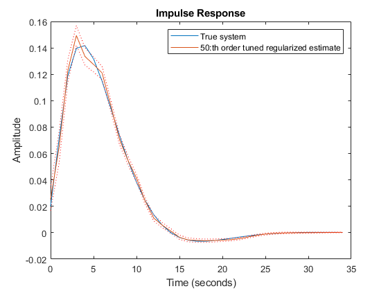
Figure 6: The true impulse response together with the tuned regularized estimate for order nb = 50.
Using Regularized ARX-Models for Estimating State-Space Models
Consider a system m0, which is a 30:th order linear system with colored measurement noise:
where G(q) is the input-to-output transfer function and H(q) is the disturbance transfer function. This system is stored in the regularizationExampleData.mat data file. The impulse responses of G(q) and H(q) are shown in Figure 7.
load regularizationExampleData.mat m0
m0H = noise2meas(m0); % the extracted noise component of the model
[yG,t] = impulse(m0);
yH = impulse(m0H,t);

clf
subplot(211)
plot(t, yG)
title('Impulse Response of G(q)'), ylabel('Amplitude')

subplot(212)
plot(t, yH)
title('Impulse Response of H(q)'), ylabel('Amplitude')
xlabel('Time (seconds)')
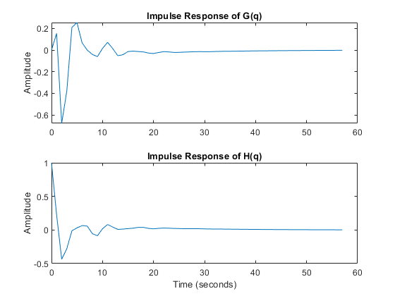
Figure 7: The impulse responses of G(q) (top) and H(q) (bottom).
We have collected 210 data points by simulating m0 with a white noise input u with variance 1, and a noise level e with variance 0.1. This data is saved in regularizationExampleData.mat and is plotted below.
load regularizationExampleData.mat m0simdata
clf
plot(m0simdata)
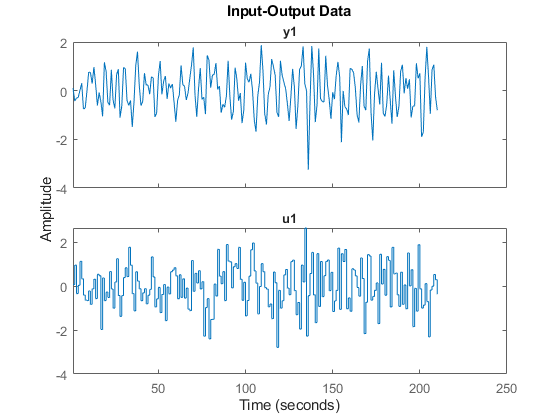
Figure 8: The data to be used for estimation.
To estimate the impulse responses of m0 from these data, we can naturally employ state-space models in the innovations form (or equivalently ARMAX models) and compute the impulse response using the impulse command as before. For computing the state-space model, we can use a syntax such as:
mk = ssest(m0simdata, k, 'Ts', 1);
The catch is to determine a good order k. There are two commonly used methods:
Cross validation CV: Estimate
mkfork = 1,...,maxousing the first half of the dataze = m0simdata(1:150)and evaluate the fit to the second half of the datazv = m0simdata(151:end)using thecomparecommand:[~,fitk] = compare(zv, mk, compareOptions('InitialCondition', 'z')). Determine the orderkthat maximizes the fit. Then reestimate the model using the whole data record.Use the Akaike criterion AIC: Estimate models for orders
k = 1,...,maxousing the whole data set, and then pick that model that minimizesaic(mk).
Applying these techniques to the data with a maximal order maxo = 30 shows that CV picks k = 15 and AIC picks k = 3.
The "Oracle" test: In addition to the CV and AIC tests, one can also check for what order k the fit between the true impulse response of G(q) (or H(q)) and the estimated model is maximized. This of course requires knowledge of the true system m0 which is impractical. However, if we do carry on this comparison for our example where m0 is known, we find that k = 12 gives the best fit of estimated model's impulse response to that of m0 (=|G(q)|). Similarly, we find that k = 3 gives the best fit of estimated model's noise component's impulse response to that of the noise component of m0 (=|H(q)|). The Oracle test sets a reference point for comparison of the quality of models generated by using various orders and regularization parameters.
Let us compare the impulse responses computed for various order selection criteria:
m3 = ssest(m0simdata, 3, 'Ts', 1);
m12 = ssest(m0simdata, 12, 'Ts', 1);
m15 = ssest(m0simdata, 15, 'Ts', 1);

y3 = impulse(m3, t);
y12 = impulse(m12, t);
y15 = impulse(m15, t);

plot(t,yG, t,y12, t,y15, t,y3)
xlabel('Time (seconds)'), ylabel('Amplitude'), title('Impulse Response')
legend('True G(q)',...
   sprintf('Oracle choice: %2.4g%%',100*(1-goodnessOfFit(y12,yG,'NRMSE'))),...
   sprintf('CV choice: %2.4g%%',100*(1-goodnessOfFit(y15,yG,'NRMSE'))),...
   sprintf('AIC choice: %2.4g%%',100*(1-goodnessOfFit(y3,yG,'NRMSE'))))

Figure 9: The true impulse response of G(q) compared to estimated models of various orders.
yH3 = impulse(noise2meas(m3), t);
yH15 = impulse(noise2meas(m15), t);

plot(t,yH, t,yH3, t,yH15, t,yH3)
xlabel('Time (seconds)'), ylabel('Amplitude'), title('Impulse Response')
legend('True H(q)',...
   sprintf('Oracle choice: %2.4g%%',100*(1-goodnessOfFit(yH3,yH,'NRMSE'))),...
   sprintf('CV choice: %2.4g%%',100*(1-goodnessOfFit(yH15,yH,'NRMSE'))),...
   sprintf('AIC choice: %2.4g%%',100*(1-goodnessOfFit(yH3,yH,'NRMSE'))))
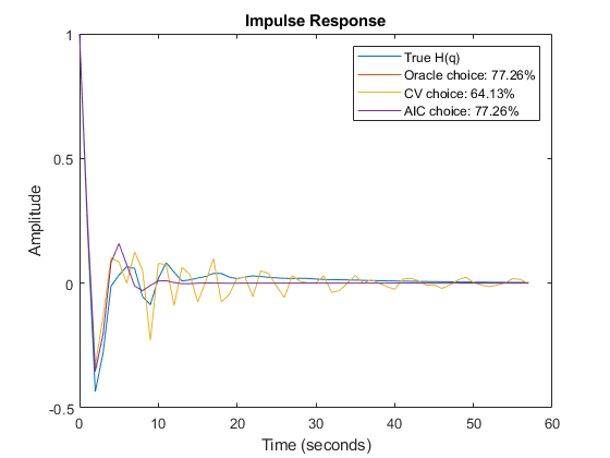
Figure 10: The true impulse response of H(q) compared to estimated noise models of various orders.
We see that a fit as good as 83% is possible to achieve for G(q) among the state-space models, but the order selection procedure may not find that best order.
We then turn to what can be obtained with regularization. We estimate a rather high order, regularized ARX-model by doing:
aopt = arxOptions;
[Lambda, R] = arxRegul(m0simdata, [5 60 0], arxRegulOptions('RegularizationKernel','TC'));
aopt.Regularization.R = R;
aopt.Regularization.Lambda = Lambda;
mr = arx(m0simdata, [5 60 0], aopt);
nmr = noise2meas(mr);
ymr = impulse(mr, t);
yHmr = impulse(nmr, t);
fprintf('Goodness of fit for ARX model is: %2.4g%%n',100*(1-goodnessOfFit(ymr,yG,'NRMSE')))
Goodness of fit for ARX model is: 83.12%n
fprintf('Goodness of fit for noise component of ARX model is: %2.4g%%n',100*(1-goodnessOfFit(yHmr,yH,'NRMSE')))
Goodness of fit for noise component of ARX model is: 78.71%n
It turns out that this regularized ARX model shows a fit to the true G(q) that is even better than the Oracle choice. The fit to H(q) is more than 80% which also is better that the Oracle choice of order for best noise model. It could be argued that mr is a high order (60 states) model, and it is unfair to compare it with lower order state space models. But this high order model can be reduced to, say, order 7 by using the balred command (requires Control System Toolbox™):
mred7 = balred(idss(mr),7);
nmred7 = noise2meas(mred7);
y7mr = impulse(mred7, t);
y7Hmr = impulse(nmred7, t);
Figures 11 and 12 show how the regularized and reduced order regularized models compare with the Oracle choice of state-space order for ssest without any loss of accuracy.
plot(t,yG, t,y12, t,ymr, t,y7mr)
xlabel('Time (seconds)'), ylabel('Amplitude'), title('Impulse Response')
legend('True G(q)',...
   sprintf('Oracle choice: %2.4g%%',100*(1-goodnessOfFit(y12,yG,'NRMSE'))),...
   sprintf('High order regularized: %2.4g%%',100*(1-goodnessOfFit(ymr,yG,'NRMSE'))),...
   sprintf('Reduced order: %2.4g%%',100*(1-goodnessOfFit(y7mr,yG,'NRMSE'))))
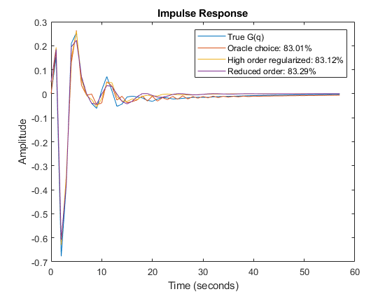
Figure 11: The regularized models compared to the Oracle choice for G(q).
plot(t,yH, t,yH3, t,yHmr, t,y7Hmr)
xlabel('Time (seconds)'), ylabel('Amplitude'), title('Impulse Response')
legend('True H(q)',...
   sprintf('Oracle choice: %2.4g%%',100*(1-goodnessOfFit(yH3,yH,'NRMSE'))),...
   sprintf('High order regularized: %2.4g%%',100*(1-goodnessOfFit(yHmr,yH,'NRMSE'))),...
   sprintf('Reduced order: %2.4g%%',100*(1-goodnessOfFit(y7Hmr,yH,'NRMSE'))))

Figure 12: The regularized models compared to the Oracle choice for H(q).
A natural question to ask is whether the choice of orders in the ARX model is as sensitive a decision as the state space model order in ssest. Simple test, using e.g. arx(z,[10 50 0], aopt), shows only minor changes in the fit of G(q).
State Space Model Estimation by Regularized Reduction Technique
The above steps of estimating a high-order ARX model, followed by a conversion to state-space and reduction to the desired order can be automated using the ssregest command. ssregest greatly simplifies this procedure while also facilitating other useful options such as search for optimal order and fine tuning of model structure by specification of feedthrough and delay values. Here we simply reestimate the reduced model similar to mred7 using ssregest:
opt = ssregestOptions('ARXOrder',[5 60 0]);
mred7_direct = ssregest(m0simdata, 7, 'Feedthrough', true, opt);
compare(m0simdata, mred7, mred7_direct)
legend(Interpreter="none")
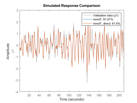
Figure 13: Comparing responses of state space models to estimation data.
h = impulseplot(mred7, mred7_direct, 40);
showConfidence(h,1) %  1 s.d. "zero interval"
hold on
s = stem(t,yG,'r');
s.DisplayName = 'True G(q)';
legend("show",Interpreter="none")
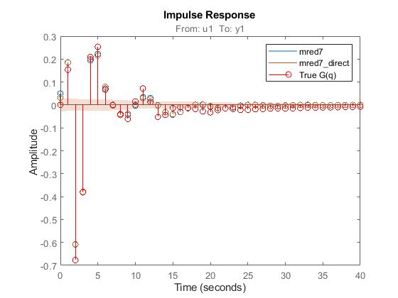
Figure 14: Comparing impulse responses of state space models.
In Figure 14, the confidence bound is only shown for the model mred7_direct since it was not calculated for the model mred7. You can use the translatecov command for generating confidence bounds for arbitrary transformations (here balred) of identified models. Note also that the ssregest command does not require you to provide the "ARXOrder" option value. It makes an automatic selection based on data length when no value is explicitly set.
Basic Bias - Variance Tradeoff in Grey Box Models
We shall discuss here grey box estimation which is a typical case where prior information meets information in observed data. It will be good to obtain a well balanced tradeoff between these information sources, and regularization is a prime tool for that.
Consider a DC motor (see e.g., iddemo7) with static gain G to angular velocity and time constant :
In state-space form we have:
where is the state vector composed of the angle and the velocity . We observe both states in noise as suggested by the output equation.
From prior knowledge and experience we think that is about 4 and is about 1. We collect in motorData 400 data points from the system, with a substantial amount of noise (standard deviation of e is 50 in each component. We also save noise-free simulation data for the same model for comparison purposes. The data is shown in Figure 15.
load regularizationExampleData.mat motorData motorData_NoiseFree
t = motorData.SamplingInstants;
subplot(311)
plot(t,[motorData_NoiseFree.y(:,1),motorData.y(:,1)])
ylabel('Output 1')
subplot(312)
plot(t,[motorData_NoiseFree.y(:,2),motorData.y(:,2)])
ylabel('Output 2')
subplot(313)
plot(t,motorData_NoiseFree.u) % input is the same for both datasets
ylabel('Input')
xlabel('Time (seconds)')
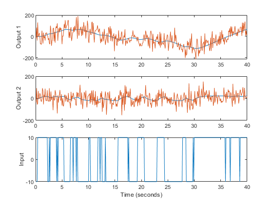
Figure 15: The noisy data to be used for grey box estimation superimposed over noise-free simulation data to be used for qualifications. From top to bottom: Angle, Angular Velocity, Input voltage.
The true parameter values in this simulation are G = 2.2 and = 0.8. To estimate the model we create an idgrey model file DCMotorODE.m.
type('DCMotorODE')function [A,B,C,D] = DCMotorODE(G,Tau,Ts) %DCMOTORODE ODE file representing the dynamics of a DC motor parameterized %by gain G and time constant Tau. % % [A,B,C,D,K,X0] = DCMOTORODE(G,Tau,Ts) returns the state space matrices % of the DC-motor with time-constant Tau and static gain G. The sample % time is Ts. % % This file returns continuous-time representation if input argument Ts % is zero. If Ts>0, a discrete-time representation is returned. % % See also IDGREY, GREYEST. % Copyright 2013 The MathWorks, Inc. A = [0 1;0 -1/Tau]; B = [0; G/Tau]; C = eye(2); D = [0;0]; if Ts>0 % Sample the model with sample time Ts s = expm([[A B]*Ts; zeros(1,3)]); A = s(1:2,1:2); B = s(1:2,3); end
An idgrey object is then created as:
mi = idgrey(@DCMotorODE,{'G', 4; 'Tau', 1},'cd',{}, 0);where we have inserted the guessed parameter value as initial values. This model is adjusted to the information in observed data by using the greyest command:
m = greyest(motorData, mi)
m =
  Continuous-time linear grey box model defined by @DCMotorODE function:
      dx/dt = A x(t) + B u(t) + K e(t)
       y(t) = C x(t) + D u(t) + e(t)

  A =
           x1      x2
   x1       0       1
   x2       0  -1.741

  B =
          u1
   x1      0
   x2  3.721

  C =
       x1  x2
   y1   1   0
   y2   0   1

  D =
       u1
   y1   0
   y2   0

  K =
       y1  y2
   x1   0   0
   x2   0   0

  Model parameters:
   G = 2.138
   Tau = 0.5745

Parameterization:
   ODE Function: @DCMotorODE
   (parametrizes both continuous- and discrete-time equations)
   Disturbance component: none
   Initial state: 'auto'
   Number of free coefficients: 2
   Use "getpvec", "getcov" for parameters and their uncertainties.

Status:
Estimated using GREYEST on time domain data "motorData".
Fit to estimation data: [29.46;4.167]%
FPE: 6.074e+06, MSE: 4908

Model Properties
The model m has the parameters = 0.57 and G = 2.14 and reproduces the data is shown in Figure 16.
copt = compareOptions('InitialCondition', 'z');
[ymi, fiti] = compare(motorData, mi, copt);
[ym, fit] = compare(motorData, m, copt);
t = motorData.SamplingInstants;
subplot(211)
plot(t, [motorData.y(:,1), ymi.y(:,1), ym.y(:,1)])
axis tight
ylabel('Output 1')
legend({'Measured output',...
   sprintf('Initial: %2.4g%%',fiti(1)),...
   sprintf('Estimated: %2.4g%%',fit(1))},...
   'Location','BestOutside')
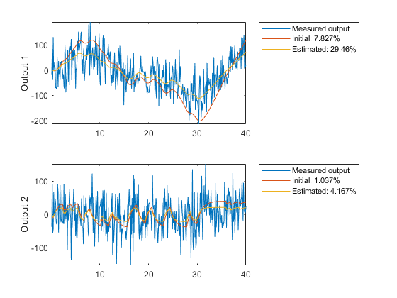
subplot(212)
plot(t, [motorData.y(:,2), ymi.y(:,2), ym.y(:,2)])
ylabel('Output 2')
axis tight
legend({'Measured output',...
   sprintf('Initial: %2.4g%%',fiti(2)),...
   sprintf('Estimated: %2.4g%%',fit(2))},...
   'Location','BestOutside')
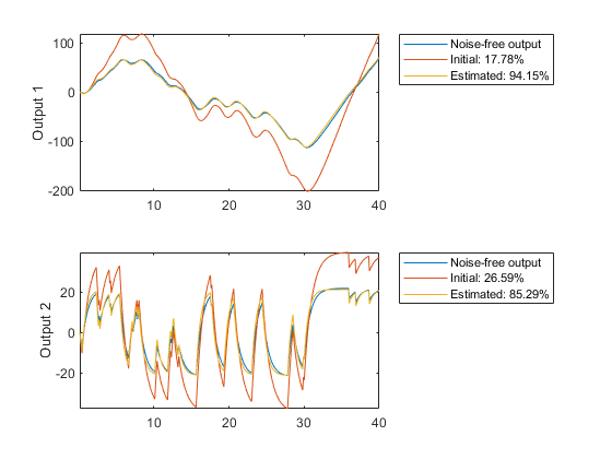
Figure 16: Measured output and model outputs for initial and estimated models.
In this simulated case we have also access to the noise-free data (motorData_NoiseFree) and depict the fit to the noise-free data in Figure 17.
[ymi, fiti] = compare(motorData_NoiseFree, mi, copt);
[ym, fit] = compare(motorData_NoiseFree, m, copt);
subplot(211)
plot(t, [motorData_NoiseFree.y(:,1), ymi.y(:,1), ym.y(:,1)])
axis tight
ylabel('Output 1')
legend({'Noise-free output',...
   sprintf('Initial: %2.4g%%',fiti(1)),...
   sprintf('Estimated: %2.4g%%',fit(1))},...
   'Location','BestOutside')
subplot(212)
plot(t, [motorData_NoiseFree.y(:,2), ymi.y(:,2), ym.y(:,2)])
ylabel('Output 2')
axis tight
legend({'Noise-free output',...
   sprintf('Initial: %2.4g%%',fiti(2)),...
   sprintf('Estimated: %2.4g%%',fit(2))},...
   'Location','BestOutside')
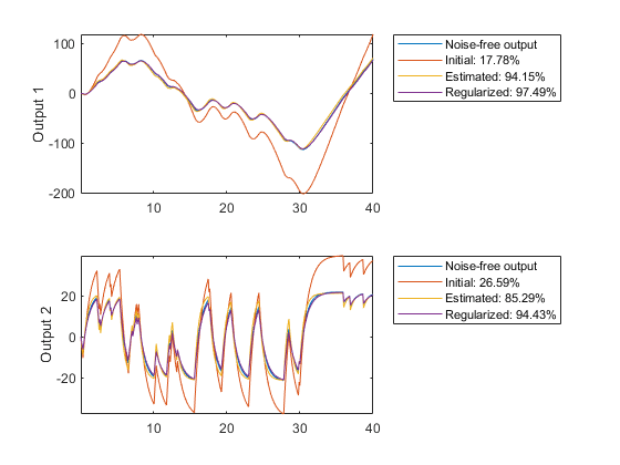
Figure 17: Noise-free output and model outputs for initial and estimated models.
We can look at the parameter estimates and see that the noisy data themselves give estimates that not quite agree with our prior physical information. To merge the data information with the prior information we use regularization:
opt = greyestOptions;
opt.Regularization.Lambda = 100;
opt.Regularization.R = [1, 1000]; % second parameter better known than first
opt.Regularization.Nominal = 'model';
mr = greyest(motorData, mi, opt)
mr =
  Continuous-time linear grey box model defined by @DCMotorODE function:
      dx/dt = A x(t) + B u(t) + K e(t)
       y(t) = C x(t) + D u(t) + e(t)

  A =
           x1      x2
   x1       0       1
   x2       0  -1.119

  B =
          u1
   x1      0
   x2  2.447

  C =
       x1  x2
   y1   1   0
   y2   0   1

  D =
       u1
   y1   0
   y2   0

  K =
       y1  y2
   x1   0   0
   x2   0   0

  Model parameters:
   G = 2.187
   Tau = 0.8938

Parameterization:
   ODE Function: @DCMotorODE
   (parametrizes both continuous- and discrete-time equations)
   Disturbance component: none
   Initial state: 'auto'
   Number of free coefficients: 2
   Use "getpvec", "getcov" for parameters and their uncertainties.

Status:
Estimated using GREYEST on time domain data "motorData".
Fit to estimation data: [29.34;3.848]%
FPE: 6.135e+06, MSE: 4933

Model Properties
We have here told the estimation process that we have some confidence in the initial parameter values, and believe more in our guess of than in our guess of G. The resulting regularized estimate mr considers this information together with the information in measured data. They are weighed together with the help of Lambda and R. In Figure 18 it is shown how the resulting model can reproduce the output. Clearly, the regularized model does a better job than both the initial model (to which the parameters are "attracted") and the unregularized model.
[ymr, fitr] = compare(motorData_NoiseFree, mr, copt);
subplot(211)
plot(t, [motorData_NoiseFree.y(:,1), ymi.y(:,1), ym.y(:,1), ymr.y(:,1)])
axis tight
ylabel('Output 1')
legend({'Noise-free output',...
   sprintf('Initial: %2.4g%%',fiti(1)),...
   sprintf('Estimated: %2.4g%%',fit(1)),...
   sprintf('Regularized: %2.4g%%',fitr(1))},...
   'Location','BestOutside')
subplot(212)
plot(t, [motorData_NoiseFree.y(:,2), ymi.y(:,2), ym.y(:,2), ymr.y(:,2)])
ylabel('Output 2')
axis tight
legend({'Noise-free output',...
   sprintf('Initial: %2.4g%%',fiti(2)),...
   sprintf('Estimated: %2.4g%%',fit(2)),...
   sprintf('Regularized: %2.4g%%',fitr(2))},...
   'Location','BestOutside')
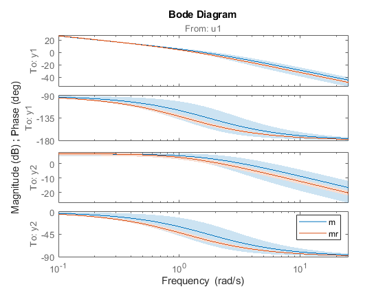
Figure 18: Noise-Free measured output and model outputs for initial, estimated and regularized models.
The regularized estimation also has reduced parameter variance as compared to the unregularized estimates. This is shown by tighter confidence bounds on the Bode plot of mr compare to that of m:
clf
showConfidence(bodeplot(m,mr,logspace(-1,1.4,100)),3) % 3 s.d. region
legend('show')
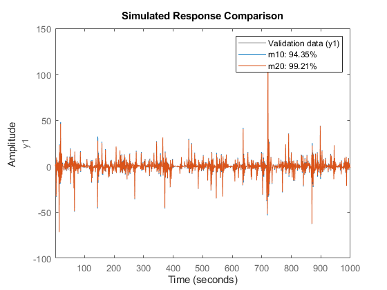
Figure 19: Bode plot of m and mr with confidence bounds
This was an illustration of how the merging prior and measurement information works. In practice we need a procedure to tune the size of Lambda to the existing information sources. A commonly used method is to use cross validation. That is:
Split the data into two parts - the estimation and the validation data
Compute the regularized model using the estimation data for various values of
LambdaEvaluate how well these models can reproduce the validation data: tabulate NRMSE fit values delivered by the
comparecommand or thegoodnessOfFitcommand.Pick that
Lambdawhich gives the model with the best fit to the validation data.
Use of Regularization to Robustify Large Nonlinear Models
Another use of regularization is to numerically stabilize the estimation of large (often nonlinear) models. We have given a data record nldata that has nonlinear dynamics. We try nonlinear ARX-model of neural network character, with more and more units:
load regularizationExampleData.mat nldata
opt = nlarxOptions('SearchMethod','lm');
m10 = nlarx(nldata, [1 2 1], idSigmoidNetwork(10), opt);
m20 = nlarx(nldata, [1 2 1], idSigmoidNetwork(20), opt);
m30 = nlarx(nldata, [1 2 1], idSigmoidNetwork(30), opt);
compare(nldata, m10, m20) % compare responses of m10, m20 to measured response 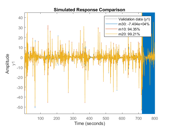
Figure 20: Comparison plot for models m10 and m20.
fprintf('Number of parameters (m10, m20, m30): %s\n',...
   mat2str([nparams(m10),nparams(m20),nparams(m30)]))
Number of parameters (m10, m20, m30): [54 104 154]
compare(nldata, m30, m10, m20) % compare all three models
axis([1 800 -57 45])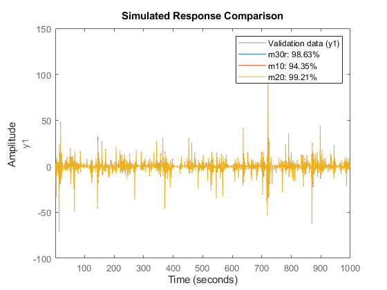
Figure 21: Comparison plot for models m10, m20 and m30.
The first two models show good and improving fits. But when estimating the 154 parameters of m30, numerical problems seem to occur. We can then apply a small amount of regularization to get better conditioned matrices:
opt.Regularization.Lambda = 1e-8;
m30r = nlarx(nldata, [1 2 1], idSigmoidNetwork(30), opt);
compare(nldata, m30r, m10, m20)

Figure 22: Comparison plot for models m10, m20 and regularized model m30r.
The fit to estimation data has significantly improved for the model with 30 neurons. As discussed before, a systematic search for the Lambda value to use would require cross validation tests.
Conclusions
We discussed the benefit of regularization for estimation of FIR models, linear grey-box models and Nonlinear ARX models. Regularization can have significant impact on the quality of the identified model provided the regularization constants Lambda and R are chosen appropriately. For ARX models, this can be done very easily using the arxRegul function. These automatic choices also feed into the dedicated state-space estimation algorithm ssregest.
For other types of estimations, you must rely on cross validation based search to determine Lambda. For structured models such as grey box models, R can be used to indicate the reliability of the corresponding initial value of the parameter. Then, using the Nominal regularization option, you can merge the prior knowledge of the parameter values with the information in the data.
Regularization options are available for all linear and nonlinear models including transfer functions and process models, state-space and polynomial models, Nonlinear ARX, Hammerstein-Wiener and linear/nonlinear grey box models.