Adjust Contrast Using Adaptive Histogram Equalization
This example shows how to adjust the contrast in an image using contrast-limited adaptive histogram equalization (CLAHE).
As an alternative to using histeq, you can perform CLAHE using the adapthisteq function. While histeq works on the entire image, adapthisteq operates on small regions in the image, called tiles. The adapthisteq function enhances the contrast of each tile, so that the histogram of the output region approximately matches a specified histogram. After performing the equalization, adapthisteq combines neighboring tiles using bilinear interpolation to eliminate artificially induced boundaries.
To avoid amplifying any noise that might be present in the image, you can use adapthisteq name-value arguments to control the tiling schema and limit the contrast, especially in homogeneous areas.
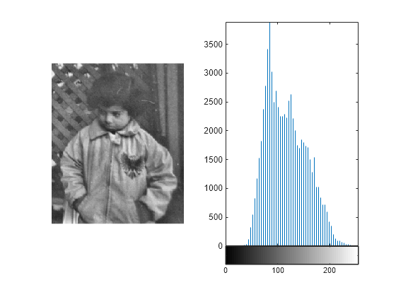
Original Image Histogram
Read an image into the workspace.
I = imread("pout.tif");View the original image and its histogram.
figure
subplot(1,2,1)
imshow(I)
subplot(1,2,2)
imhist(I,64)

Adjust Contrast Using Default Adaptive Equalization
Adjust the contrast of the image using adaptive histogram equalization. By default, adapthisteq divides the image into an 8-by-8 tile grid, and adjusts each tile using a uniform distribution with 256 bins and a clip limit of 0.01.
J = adapthisteq(I);
Display the contrast-adjusted image with its histogram.
figure
subplot(1,2,1)
imshow(J)
subplot(1,2,2)
imhist(J,64)
Adjust Contrast by Specifying Number of Tiles
Adjust the contrast, specifying a different number of tiles. Increasing the number of tiles results in more localized contrast enhancement, and can lead to more noticeable boundaries between tiles.
numTiles =
20
20numTiles = 20
J = adapthisteq(I,NumTiles=[numTiles numTiles]);
Display the contrast-adjusted image and its new histogram.
figure
subplot(1,2,1)
imshow(J)
subplot(1,2,2)
imhist(J,64)

Adjust Contrast by Specifying Clip Limit
Adjust the contrast, specifying a different clip limit. The clip limit controls the amount of contrast enhancement in each tile, preventing oversaturation and noise amplification. You can specify a clip limit in the range [0, 1] using the ClipLimit name-value argument. A value closer to 1 results in more contrast enhancement, at the risk of amplifying noise. The default value is 0.01.
clipLim = 0.03;
J = adapthisteq(I,ClipLimit=clipLim);
0.03;
J = adapthisteq(I,ClipLimit=clipLim);Display the contrast-adjusted image with its histogram. Using a clip limit of 0.03, the image has greater contrast and a more uniform distribution compared to the default clip limit.
figure
subplot(1,2,1)
imshow(J)
subplot(1,2,2)
imhist(J,64)

Adjust Contrast by Specifying Target Distribution
Adjust the contrast, specifying the target distribution for each tile. By default, the function targets a uniform distribution, which tends to maximize contrast over the full range of intensity values. Alternatively, you can specify an exponential or Rayleigh distribution, which both tend to enhance lower-intensity values more than brighter values. The distribution you select typically depends on the input image type. For example, the Rayleigh distribution tends to preserve the natural appearance of the image, and is therefore common for medical or underwater images. For the exponential and Rayleigh distributions, you can further adjust the shape of the distribution by specifying the Alpha name-value argument.
dist =
"rayleigh"
dist = "rayleigh"
J = adapthisteq(I,Distribution=dist);

figure
subplot(1,2,1)
imshow(J)
subplot(1,2,2)
imhist(J,64)

Adjust Contrast by Specifying Number of Bins
Adjust the contrast, specifying a different number of bins. With a smaller number of bins, the adapthisteq function uses fewer gray levels to display the contrast-adjusted image. Increasing the number of bins increases the dynamic range of the image, at the cost of slower processing speed.
nbins = 20;
J = adapthisteq(I,NBins=nbins);
figure
subplot(1,2,1)
imshow(J)
subplot(1,2,2)
imhist(J,64)
20;
J = adapthisteq(I,NBins=nbins);
figure
subplot(1,2,1)
imshow(J)
subplot(1,2,2)
imhist(J,64)