Lane Detection in 3-D Lidar Point Cloud

Open Live Script

This example shows how to detect lanes in lidar point clouds. You can use the intensity values returned from lidar point clouds to detect ego vehicle lanes. You can further improve the lane detection by using a curve-fitting algorithm and tracking the curve parameters. Lidar lane detection enables you to build complex workflows like lane keep assist, lane departure warning, and adaptive cruise control for autonomous driving. A test vehicle collects the lidar data using a lidar sensor mounted on its rooftop.

Introduction

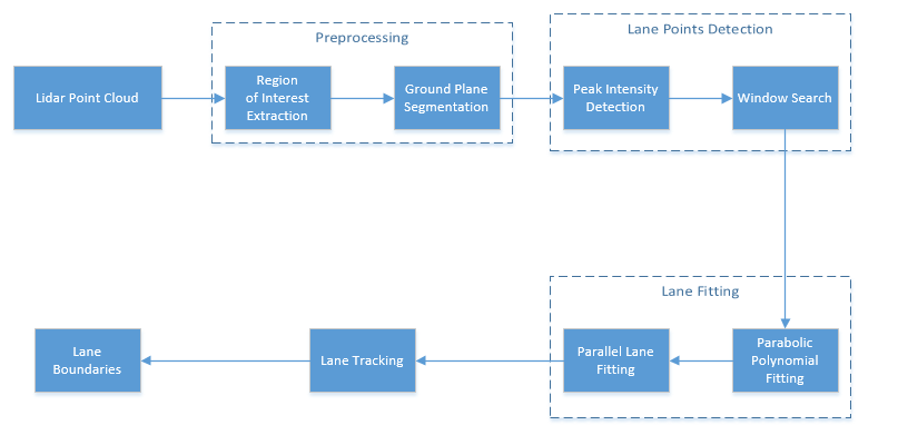
Lane detection in lidar involves detection of the immediate left and right lanes, also known as ego vehicle lanes, with respect to the lidar sensor. It involves the following steps:

Region of interest extraction
Ground plane segmentation
Peak intensity detection
Lane detection using window search
Parabolic polynomial fitting
Parallel lane fitting
Lane tracking

This flowchart gives an overview of the workflow presented in this example.

The advantages of using lidar data for lane detection are :

Lidar point clouds give a better 3-D representation of the road surface than image data, thus reducing the required calibration parameters to find the bird's-eye view.
Lidar is more robust against adverse climatic conditions than image-based detection.
Lidar data has a centimeter level of accuracy, leading to accurate lane localization.

Download and Prepare Lidar Data Set

The lidar data used in this example has been collected using the Ouster OS1-64 channel lidar sensor, producing high-resolution point clouds. This data set contains point clouds stored as a cell array of pointCloud object. Each 3-D point cloud consists of XYZ locations along with intensity information.

Note: Download time of the data depends on your internet connection. MATLAB will be temporarily unresponsive during the execution of this code block.

% Download lidar data
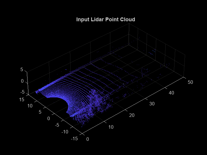
lidarData = helperGetDataset;

Selecting the first frame of the dataset for further processing.

% Select first frame 
ptCloud = lidarData{1};

% Visualize input point cloud
figure
pcshow(ptCloud,ColorSource="Intensity")
title('Input Lidar Point Cloud')
axis([0 50 -15 15 -5 5])
view([-42 35])

Figure contains an axes object. The axes object with title Input Lidar Point Cloud contains an object of type scatter.

Preprocessing

To estimate the lane points, first preprocess the lidar point clouds. Preprocessing involves the following steps:

Region of interest extraction
Ground plane segmentation

% Define ROI in meters
xlim = [5 55];
ylim = [-3 3];
zlim = [-4 1];
roi = [xlim ylim zlim];

% Crop point cloud using ROI
indices = findPointsInROI(ptCloud,roi);
croppedPtCloud = select(ptCloud,indices);

% Remove ground plane
maxDistance = 0.1;
referenceVector = [0 0 1];
[model,inliers,outliers] = pcfitplane(croppedPtCloud,maxDistance,referenceVector);
groundPts = select(croppedPtCloud,inliers);

figure
pcshow(groundPts,ColorSource="Intensity")
title('Ground Plane')
view(3)

Figure contains an axes object. The axes object with title Ground Plane contains an object of type scatter.

Lane Point Detection

Detect lane points by using a sliding window search, where the initial estimates for the sliding windows are made using an intensity-based histogram.

Lane point detection consists primarily of these two steps:

Peak intensity detection
Window search

Peak Intensity Detection

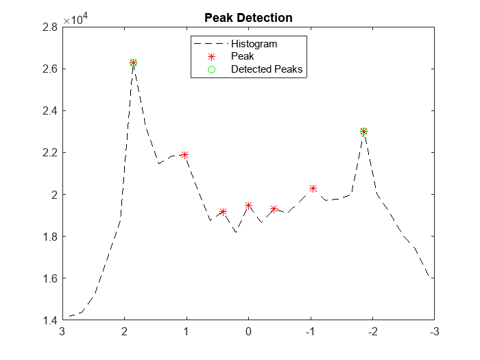
Lane points in the lidar point cloud have a distinct distribution of intensities. Usually, these intensities occupy the upper region in the histogram distribution and appear as high peaks. Compute a histogram of intensities from the detected ground plane along the ego vehicle axis (positive X-axis). The helperComputeHistogram helper function creates a histogram of intensity points. Control the number of bins for the histogram by specifying the bin resolution.

histBinResolution = 0.2;
[histVal,yvals] = helperComputeHistogram(groundPts,histBinResolution);

figure
plot(yvals,histVal,'--k')
set(gca,'XDir','reverse')
hold on

Obtain peaks in the histogram by using the helperfindpeaks helper function. Further filter the possible lane points based on lane width using the helperInitialWindow helper function.

[peaks,locs] = helperfindpeaks(histVal);
startYs = yvals(locs);

laneWidth = 4;
[startLanePoints,detectedPeaks] = helperInitialWindow(startYs,peaks,laneWidth);

plot(startYs,peaks,'*r')
plot(startLanePoints,detectedPeaks,'og')
legend('Histogram','Peak','Detected Peaks','Location','North')
title('Peak Detection')
hold off

Figure contains an axes object. The axes object with title Peak Detection contains 3 objects of type line. One or more of the lines displays its values using only markers These objects represent Histogram, Peak, Detected Peaks.

Window Search

Window search is used to detect lane points by sliding the windows along the lane curvature direction. Window search consists of two steps:

Window initialization
Sliding window

Window Initialization

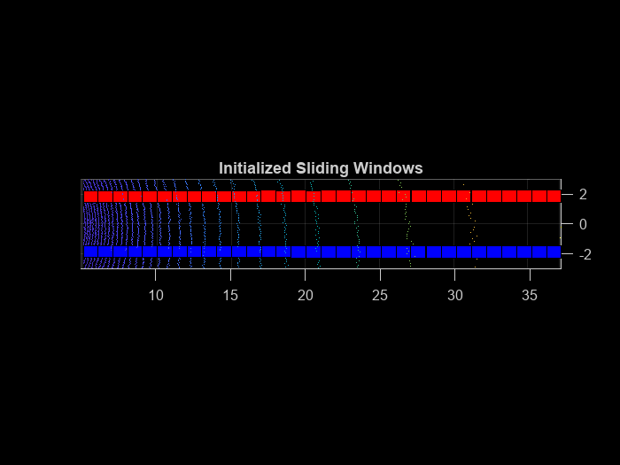
The detected peaks help in the initialization of the search window. Initialize the search windows as multiple bins with red and blue colors for left and right lanes respectively.

vBinRes = 1;
hBinRes = 0.8;
numVerticalBins = ceil((groundPts.XLimits(2) - groundPts.XLimits(1))/vBinRes);
laneStartX = linspace(groundPts.XLimits(1),groundPts.XLimits(2),numVerticalBins);

% Display bin windows
figure
pcshow(groundPts)
view(2)
helperDisplayBins(laneStartX,startLanePoints(1),hBinRes/2,groundPts,'red');
helperDisplayBins(laneStartX,startLanePoints(2),hBinRes/2,groundPts,'blue');
title('Initialized Sliding Windows')

Figure contains an axes object. The axes object with title Initialized Sliding Windows contains 65 objects of type scatter, patch.

Sliding Window

The sliding bins are initialized from the bin locations, and iteratively move along the ego vehicle (positive X-axis) direction. The helperDetectLanes helper function detects lane points and visualizes the sliding bins. Consecutive bins slide along the Y-axis based upon the intensity values inside the previous bin.

At regions where the lane points are missing, the function predicts the sliding bins using second-degree polynomial. This condition commonly arises when there are moving object's crossing the lanes. The sliding bins are yellow and the bins that are predicted using the polynomial are green.

display = true;
lanes = helperDetectLanes(groundPts,hBinRes, ...
    numVerticalBins,startLanePoints,display);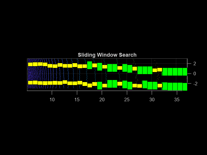

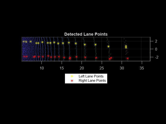
Figure contains an axes object. The axes object with title Sliding Window Search contains 65 objects of type scatter, patch.

% Plot final lane points
lane1 = lanes{1};
lane2 = lanes{2};

figure
pcshow(groundPts)
title('Detected Lane Points')
hold on
p1 = plot3(lane1(:,1),lane1(:,2),lane1(:,3),'*y');
p2 = plot3(lane2(:,1),lane2(:,2),lane2(:,3),'*r');
hold off
view(2)
lgnd = legend([p1 p2],{'Left Lane Points','Right Lane Points'});
set(lgnd,'color','White','Location','southoutside')

Figure contains an axes object. The axes object with title Detected Lane Points contains 3 objects of type scatter, line. One or more of the lines displays its values using only markers These objects represent Left Lane Points, Right Lane Points.

Lane Fitting

Lane fitting involves estimating a polynomial curve on the detected lane points. These polynomials are used along with parallel lane constraint for lane fitting.

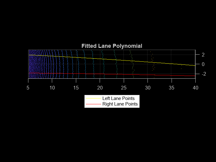
Parabolic Polynomial Fitting

The polynomial is fitted on X-Y points using a 2-degree polynomial represented as $a x^{2} + bx + c$ , where a, b, and c are polynomial parameters. To perform curve fitting, use the helperFitPolynomial helper function, which also handles outliers using the random sample consensus (RANSAC) algorithm. To estimate the 3-D lane points, extract the parameters from the plane model created during the preprocessing step. The plane model is represented as $ax + by + cz + d = 0$ , where the Z-coordinate is unknown. Estimate the Z-coordinate by substituting the X- and Y-coordinates in the plane equation.

[P1,error1] = helperFitPolynomial(lane1(:,1:2),2,0.1);
[P2,error2] = helperFitPolynomial(lane2(:,1:2),2,0.1);

xval = linspace(5,40,80);
yval1 = polyval(P1,xval);
yval2 = polyval(P2,xval);

% Z-coordinate estimation
modelParams = model.Parameters;
zWorld1 = (-modelParams(1)*xval - modelParams(2)*yval1 - modelParams(4))/modelParams(3);
zWorld2 = (-modelParams(1)*xval - modelParams(2)*yval2 - modelParams(4))/modelParams(3);

% Visualize fitted lane
figure
pcshow(croppedPtCloud)
title('Fitted Lane Polynomial')
hold on
p1 = plot3(xval,yval1,zWorld1,'y','LineWidth',0.2);
p2 = plot3(xval,yval2,zWorld2,'r','LineWidth',0.2);
lgnd = legend([p1 p2],{'Left Lane Points','Right Lane Points'});
set(lgnd,'color','White','Location','southoutside')
view(2)
hold off

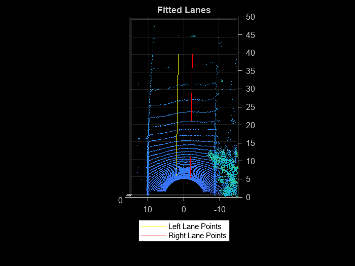
Figure contains an axes object. The axes object with title Fitted Lane Polynomial contains 3 objects of type scatter, line. These objects represent Left Lane Points, Right Lane Points.

Parallel Lane Fitting

The lanes are usually parallel to each other along the road. To make the lane fitting robust, use this parallel constraint. When fitting the polynomials, the helperFitPolynomial helper function also computes, the fitting error. Update the lanes having erroneous points with the new polynomial. Update this polynomial by shifting it along the Y-axis.

lane3d1 = [xval' yval1' zWorld1'];
lane3d2 = [xval' yval2' zWorld2'];

% Shift the polynomial with a high score along the Y-axis towards
% the polynomial with a low score
if error1 > error2
    lanePolynomial = P2;
    if lane3d1(1,2) > 0
        lanePolynomial(3) = lane3d2(1,2) + laneWidth;
    else
        lanePolynomial(3) = lane3d2(1,2) - laneWidth;
    end
    lane3d1(:,2) = polyval(lanePolynomial,lane3d1(:,1));
    lanePolynomials = [lanePolynomial; P2];
else
    lanePolynomial = P1;
    if lane3d2(1,2) > 0
        lanePolynomial(3) = lane3d1(1,2) + laneWidth;
    else
        lanePolynomial(3) = lane3d1(1,2) - laneWidth;
    end
    lane3d2(:,2) = polyval(lanePolynomial,lane3d2(:,1));
    lanePolynomials = [P1; lanePolynomial]
end

% Visualize lanes after parallel fitting
figure
pcshow(ptCloud)
axis([0 50 -15 15 -5 5])
hold on
p1 = plot3(lane3d1(:,1),lane3d1(:,2),lane3d1(:,3),'y','LineWidth',0.2);
p2 = plot3(lane3d2(:,1),lane3d2(:,2),lane3d2(:,3),'r','LineWidth',0.2);
view([-90 90])
title('Fitted Lanes')
lgnd = legend([p1 p2],{'Left Lane Points','Right Lane Points'});
set(lgnd,'color','White','Location','southoutside')
hold off

Figure contains an axes object. The axes object with title Fitted Lanes contains 3 objects of type scatter, line. These objects represent Left Lane Points, Right Lane Points.

Lane Tracking

Lane tracking helps in stabilizing the lane curvature caused by sudden jerks and drifts. These changes can occur because of missing lane points, vehicles moving over the lanes, and erroneous lane detection. Lane tracking is a two-step process:

Track lane polynomial parameters $(a, b)$ to control the curvature of the polynomial.
Track the start points coming from peak detection. This parameter is denoted as $c$ in the polynomial.

These parameters are updated using a Kalman filter with a constant acceleration motion model. To initiate a Kalman filter, use the configureKalmanFilter.

% Initial values
curveInitialParameters = lanePolynomials(1,1:2);
driftInitialParameters = lanePolynomials(:,3)';
initialEstimateError = [1 1 1]*1e-1;
motionNoise = [1 1 1]*1e-7;
measurementNoise = 10;

% Configure Kalman filter
curveFilter = configureKalmanFilter('ConstantAcceleration', ...
    curveInitialParameters,initialEstimateError,motionNoise,measurementNoise);
driftFilter = configureKalmanFilter('ConstantAcceleration', ...
    driftInitialParameters,initialEstimateError,motionNoise,measurementNoise);

Loop Through Data

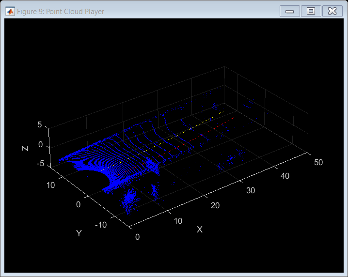
Loop through and process the lidar data by using the helperLaneDetector helper class. This helper class implements all previous steps, and also performs additional preprocessing to remove the vehicles from the point cloud. This ensures that the detected ground points are flat and the plane model is accurate. The class method detectLanes detects and extracts the lane points for the left and right lane as a two-element cell array, where the first element corresponds to the left lane and the second element to the right lane.

% Initialize the random number generator
rng(2020)
numFrames = numel(lidarData);
detector = helperLaneDetector('ROI',[5 40 -3 3 -4 1]);

% Turn on display
player = pcplayer([0 50],[-15 15],[-5 5]);

drift = zeros(numFrames,1);
filteredDrift = zeros(numFrames,1);
curveSmoothness = zeros(numFrames,1);
filteredCurveSmoothness = zeros(numFrames,1);
for i = 1:numFrames
    ptCloud = lidarData{i};

    % Detect lanes
    detectLanes(detector,ptCloud);

    % Predict polynomial from Kalman filter
    predict(curveFilter);
    predict(driftFilter);

    % Correct polynomial using Kalman filter
    lanePolynomials = detector.LanePolynomial;
    drift(i) = mean(lanePolynomials(:,3));
    curveSmoothness(i) = mean(lanePolynomials(:,1));
    updatedCurveParams = correct(curveFilter,lanePolynomials(1,1:2));
    updatedDriftParams = correct(driftFilter,lanePolynomials(:,3)');

    % Update lane polynomials
    updatedLanePolynomials = [repmat(updatedCurveParams,[2 1]),updatedDriftParams'];

    % Estimate new lane points with updated polynomial
    lanes = updateLanePolynomial(detector,updatedLanePolynomials);
    filteredDrift(i) = mean(updatedLanePolynomials(:,3));
    filteredCurveSmoothness(i) = mean(updatedLanePolynomials(:,1));

    % Visualize lanes after parallel fitting
    ptCloud.Color = uint8(repmat([0 0 255],ptCloud.Count,1));
    lane3dPc1 = pointCloud(lanes{1});
    lane3dPc1.Color = uint8(repmat([255 0 0],lane3dPc1.Count,1));
    lanePc = pccat([ptCloud lane3dPc1]);
    lane3dPc2 = pointCloud(lanes{2});
    lane3dPc2.Color = uint8(repmat([255 255 0],lane3dPc2.Count,1));
    lanePc = pccat([lanePc lane3dPc2]);
    view(player,lanePc)
end

Figure Point Cloud Player contains an axes object. The axes object with xlabel X, ylabel Y contains an object of type scatter.

Results

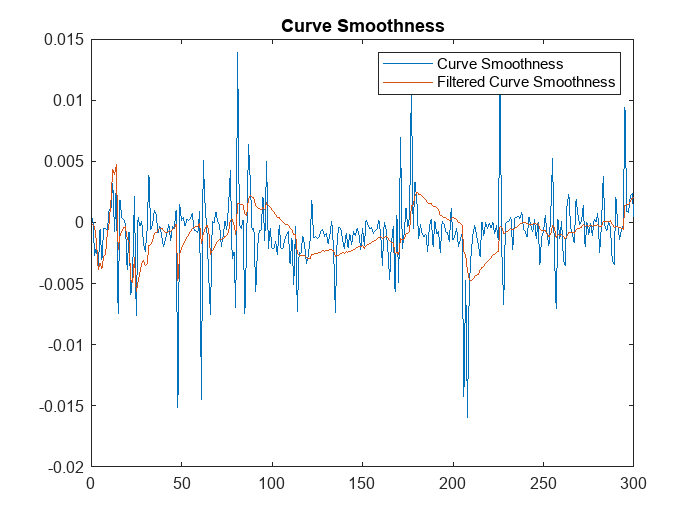
To analyze the lane detection results, compare them against the tracked lane polynomials by plotting them in figures. Each plot compares the parameters with and without the Kalman filter. The first plot compares the drift of lanes along the Y-axis, and the second plot compares the smoothness of the lane polynomials. Smoothness is defined as the rate of change of the slope of the lane curve.

figure
plot(drift)
hold on
plot(filteredDrift)
hold off
title('Lane Drift Along Y-axis')
legend('Drift Values','Filtered Drift Values')

Figure contains an axes object. The axes object with title Lane Drift Along Y-axis contains 2 objects of type line. These objects represent Drift Values, Filtered Drift Values.

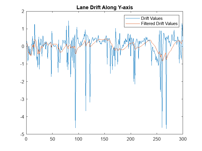
figure
plot(curveSmoothness)
hold on
plot(filteredCurveSmoothness)
hold off
title('Curve Smoothness')
legend('Curve Smoothness','Filtered Curve Smoothness')

Figure contains an axes object. The axes object with title Curve Smoothness contains 2 objects of type line. These objects represent Curve Smoothness, Filtered Curve Smoothness.

Summary

This example has shown you how to detect lanes on the intensity channel of point clouds coming from lidar sensor. You have also learned how to fit a 2-D polynomial on detected lane points, and leverage ground plane model to estimate 3-D lane points. You have also used Kalman filter tracking to further improve lane detection.

Supporting Functions

The helperLoadData helper function loads the lidar data set into the MATLAB workspace.

function reflidarData = helperGetDataset()
lidarDataTarFile = matlab.internal.examples.downloadSupportFile( ...
    'lidar','data/WPI_LidarData.tar.gz');
[outputFolder,~,~] = fileparts(lidarDataTarFile);

% Check if tar.gz file is downloaded, but not uncompressed
if ~exist(fullfile(outputFolder,'WPI_LidarData.mat'),'file')
    untar(lidarDataTarFile,outputFolder);
end

% Load lidar data
load(fullfile(outputFolder,'WPI_LidarData.mat'),'lidarData');

% Select region with a prominent intensity value
reflidarData = cell(300,1);
count = 1;
roi = [-50 50 -30 30 -inf inf];
for i = 81:380
    pc = lidarData{i};
    ind = findPointsInROI(pc,roi);
    reflidarData{count} = select(pc,ind);
    count = count+1;
end
end

This helperInitialWindow helper function computes the starting points of the search window using the detected histogram peaks.

function [yval,detectedPeaks] = helperInitialWindow(yvals,peaks,laneWidth)
leftLanesIndices = yvals >= 0;
rightLanesIndices = yvals < 0;
leftLaneYs = yvals(leftLanesIndices);
rightLaneYs = yvals(rightLanesIndices);
peaksLeft = peaks(leftLanesIndices);
peaksRight = peaks(rightLanesIndices);
diff = zeros(sum(leftLanesIndices),sum(rightLanesIndices));
for i = 1:sum(leftLanesIndices)
    for j = 1:sum(rightLanesIndices)
        diff(i,j) = abs(laneWidth - (leftLaneYs(i) - rightLaneYs(j)));
    end
end
[~,minIndex] = min(diff(:));
[row,col] = ind2sub(size(diff),minIndex);
yval = [leftLaneYs(row) rightLaneYs(col)];
detectedPeaks = [peaksLeft(row) peaksRight(col)];
estimatedLaneWidth = leftLaneYs(row) - rightLaneYs(col);

% If the calculated lane width is not within the bounds,
% return the lane with highest peak
if abs(estimatedLaneWidth - laneWidth) > 0.5
    if max(peaksLeft) > max(peaksRight)
        yval = [leftLaneYs(maxLeftInd) NaN];
        detectedPeaks = [peaksLeft(maxLeftInd) NaN];
    else
        yval = [NaN rightLaneYs(maxRightInd)];
        detectedPeaks = [NaN rightLaneYs(maxRightInd)];
    end
end
end

This helperFitPolynomial helper function fits a RANSAC-based polynomial to the detected lane points and computes the fitting score.

function [P,score] = helperFitPolynomial(pts,degree,resolution)
P = fitPolynomialRANSAC(pts,degree,resolution);
ptsSquare = (polyval(P,pts(:,1)) - pts(:,2)).^2;
score =  sqrt(mean(ptsSquare));
end

This helperComputeHistogram helper function computes the histogram of the intensity values of the point clouds.

function [histVal,yvals] = helperComputeHistogram(ptCloud,histogramBinResolution)
numBins = ceil((ptCloud.YLimits(2) - ptCloud.YLimits(1))/histogramBinResolution);
histVal = zeros(1,numBins-1);
binStartY = linspace(ptCloud.YLimits(1),ptCloud.YLimits(2),numBins);
yvals = zeros(1,numBins-1);
for i = 1:numBins-1
    roi = [-inf 15 binStartY(i) binStartY(i+1) -inf inf];
    ind = findPointsInROI(ptCloud,roi);
    subPc = select(ptCloud,ind);
    if subPc.Count
        histVal(i) = sum(subPc.Intensity);
        yvals(i) = (binStartY(i) + binStartY(i+1))/2;
    end
end
end

This helperfindpeaks helper function extracts peaks from the histogram values.

function [pkHistVal,pkIdx] = helperfindpeaks(histVal)
pkIdxTemp = (1:size(histVal,2))';
histValTemp = [NaN; histVal'; NaN];
tempIdx = (1:length(histValTemp)).';

% keep only the first of any adjacent pairs of equal values (including NaN)
yFinite = ~isnan(histValTemp);
iNeq = [1; 1 + find((histValTemp(1:end-1) ~= histValTemp(2:end)) & ...
    (yFinite(1:end-1) | yFinite(2:end)))];
tempIdx = tempIdx(iNeq);

% Take the sign of the first sample derivative
s = sign(diff(histValTemp(tempIdx)));

% Find local maxima
maxIdx = 1 + find(diff(s) < 0);

% Index into the original index vector without the NaN bookend
pkIdx = tempIdx(maxIdx) - 1;

% Fetch the coordinates of the peak
pkHistVal = histVal(pkIdx);
pkIdx = pkIdxTemp(pkIdx)';
end

References

[1] Ghallabi, Farouk, Fawzi Nashashibi, Ghayath El-Haj-Shhade, and Marie-Anne Mittet. "LIDAR-Based Lane Marking Detection for Vehicle Positioning in an HD Map." In 2018 21st International Conference on Intelligent Transportation Systems (ITSC), 2209-14. Maui: IEEE, 2018. https://doi.org/10.1109/ITSC.2018.8569951.

[2] Thuy, Michael and Fernando León. "Lane Detection and Tracking Based on Lidar Data." Metrology and Measurement Systems 17, no. 3 (2010): 311-322. https://doi.org/10.2478/v10178-010-0027-3.