Motion Compensation in 3-D Lidar Point Clouds Using Sensor Fusion

This example uses:

This example shows how to compensate point cloud distortion due to ego vehicle motion by fusing data from Global Positioning System (GPS) and inertial measurement unit (IMU) sensors. The goal of this example is to compensate the distortion in the point cloud data and recreate the surroundings accurately.

Overview

Ego vehicle motion induces distortion in the point cloud data collected from the attached lidar sensor. The extent of distortion depends on the ego vehicle velocity and the scan rate of the lidar sensor. A mechanical lidar sensor scans the environment by rotating a mirror that reflects laser pulses and generates point cloud data of the surrounding environment. The rotational speed of this mirror determines the scan rate of the sensor. Lidar sensors generate point cloud data assuming that each measurement is captured from the same viewpoint, but the ego vehicle motion changes the mirror rotation, thereby changing the viewpoint at which the sensor captures data. This difference between assumed and actual viewpoint causes distortion in the generated point cloud.

This figure shows the top view of how the distortion occurs when the ego vehicle is moving and how to compensate it by using the ego vehicle pose at each point in the point cloud.

Existing motion compensation algorithms use either point cloud data, or dedicated sensors like GPS and IMU, to estimate ego vehicle motion. This example uses the GPS and IMU sensor approach. The algorithm assumes that the data from the GPS and IMU sensors is accurate and fuses them to obtain the odometry of the ego vehicle. Then, the algorithm adjusts each point in the point cloud by interpolating the vehicle odometry.

This example uses Udacity® data recorded using GPS, IMU, camera, and lidar sensors. This example follows these steps to compensate for the motion distortion in the recorded point cloud data.

Preprocess and align the data.
Fuse GPS and IMU sensor data.
Align fused data in the east-north-up (ENU) frame.
Correct distortion in the point cloud data.

Download Data

For this example, recorded ego vehicle data has been collected from the Udacity data set and stored as a .mat file. The recorded data includes:

GPS data — Contains the latitude, longitude, altitude, and velocity of the ego vehicle at each GPS timestamp.
IMU data — Contains the linear acceleration and angular velocity of the ego vehicle at each IMU timestamp.
Lidar data — Contains the point cloud data of the environment at each lidar timestamp, saved as a pointCloud object.

Note: The download time of the data depends on your internet connection. MATLAB will be temporarily unresponsive during the execution of this code block.

% Load GPS data into the workspace
gpsZipFile = matlab.internal.examples.downloadSupportFile("driving", ...
    "data/UdacityHighway/gps.zip");
outputFolder = fileparts(gpsZipFile);
gpsFile = fullfile(outputFolder,"gps/gps.mat");
if ~exist(gpsFile,"file")
    unzip(gpsZipFile,outputFolder)
end
load(gpsFile)

% Load IMU data into the workspace
imuZipFile = matlab.internal.examples.downloadSupportFile("driving", ...
    "data/UdacityHighway/imu.zip");
outputFolder = fileparts(imuZipFile);
imuFile = fullfile(outputFolder,"imu/imu.mat");
if ~exist(imuFile,"file")
    unzip(imuZipFile,outputFolder)
end
load(imuFile)

% Load lidar data into the workspace
lidarZipFile = matlab.internal.examples.downloadSupportFile("driving", ...
    "data/UdacityHighway/lidar.zip");
outputFolder = fileparts(lidarZipFile);
lidarFile = fullfile(outputFolder,"lidar/lidar.mat");
if ~exist(lidarFile,"file")
    unzip(lidarZipFile,outputFolder)
end
load(lidarFile)

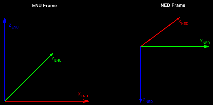
Coordinate System

In this example, the GPS and lidar sensor data is in the ENU frame of reference, and the IMU sensor data is in the north-east-down (NED) frame of reference.

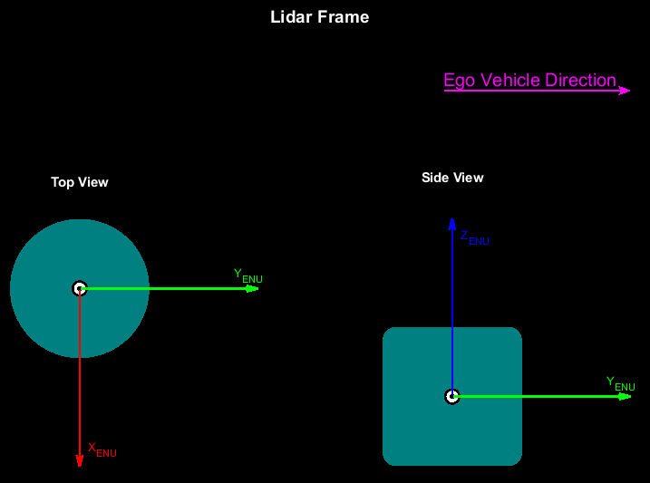
In the lidar frame, the y-axis points in the direction of ego-vehicle motion, x-axis points to the right, and z-axis points upward from the ground.

This example converts all the sensor data into the ego-vehicle coordinate system to adjust the point cloud data. The vehicle coordinate system is anchored to the ego vehicle and follows the ISO 8855 convention for rotation. This coordinate system is in the ENU frame. The origin of the vehicle coordinate system is the roof center of the ego vehicle.

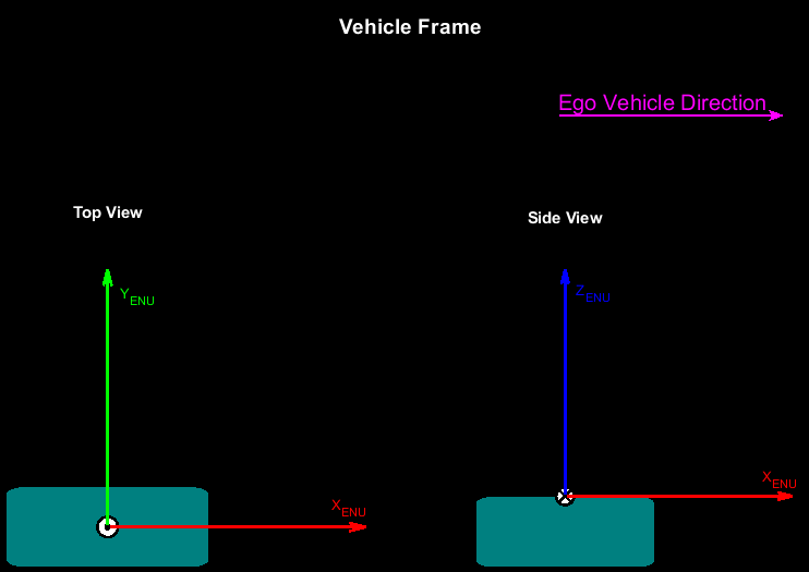
This example assumes the raw data of all sensors has already been transformed to the ego-vehicle center. This is how the sensors are aligned with respect to the vehicle coordinate system.

The GPS data is in the vehicle coordinate system.
The IMU data is in the vehicle coordinate system in the NED frame.
The lidar data is in the vehicle coordinate system with a yaw angle of 90 degrees counterclockwise.

If you are using data in which any of these assumptions are not met, then you must transform the data to satisfy the assumptions before proceeding further in this example.

Preprocess Lidar Data

Select point cloud frames for motion compensation, and transform them from the lidar ENU frame to the vehicle ENU frame.

% Transform from lidar ENU to vehicle ENU
rot = [0 0 -90];
trans = [0 0 0];
tform = rigidtform3d(rot,trans);

% Select point cloud frames for motion compensation
lidarFrames = 45:54;

% Define variable to hold selected point cloud frames
lidarData = lidar.PointCloud;
lidarDataAlign = lidarData(lidarFrames);

% Align selected point cloud frames
for frameId = 1:numel(lidarDataAlign)
    lidarDataAlign(frameId) = pctransform(lidarDataAlign(frameId),tform);
end

Preprocess GPS Data

Use the latlon2local (Automated Driving Toolbox) function to convert the raw GPS coordinates to the vehicle ENU frame. These coordinates give the waypoints of the ego vehicle trajectory.

% Convert raw GPS coordinates to vehicle ENU frame
gpsStartLocation = [gps.Latitude(1,1) gps.Longitude(1,1) gps.Altitude(1,1)];
[currentEast,currentNorth,currentUp] = latlon2local(gps.Latitude,gps.Longitude, ...
    gps.Altitude,gpsStartLocation);
waypointsGPS = [currentEast currentNorth currentUp];

To fuse the GPS and IMU sensor data, transform the waypoints into the IMU frame.

waypoints = [waypointsGPS(:,2) waypointsGPS(:,1) -1*waypointsGPS(:,3)];

Combine GPS, IMU, and Lidar Data

The GPS, IMU, and lidar data is in the timetable format. Combine the data together into one matrix, inputDataMatrix, for use in fusion.

% Create a table with synchronized GPS, IMU and Lidar sensor data
gpsTable = timetable(gps.Time,[gps.Latitude gps.Longitude gps.Altitude],gps.Velocity);
gpsTable.Properties.VariableNames(1) = "GPSPosition";
gpsTable.Properties.VariableNames(2) = "GPSVelocity";
imuTable = timetable(imu.Time,imu.LinearAcceleration,imu.AngularVelocity);
imuTable.Properties.VariableNames(1) = "Accelerometer";
imuTable.Properties.VariableNames(2) = "Gyroscope";
lidarTable = timetable(lidar.Time,ones(size(lidar.Time,1),1));
lidarTable.Properties.VariableNames(1) = "LidarFlag";
inputDataMatrix = synchronize(gpsTable,imuTable,lidarTable);

Fuse GPS and IMU Sensor Data

This example uses a Kalman filter to asynchronously fuse the GPS and IMU data by using an insfilterAsync (Navigation Toolbox) object.

% Create an INS filter to fuse asynchronous GPS and IMU data
filt = insfilterAsync(ReferenceFrame="NED");

Define the measurement covariance error for each sensor. This example obtains error parameters using experimentation, and by autotuning an insfilterAsync (Navigation Toolbox) object. For more information, see Automatic Tuning of the insfilterAsync Filter (Navigation Toolbox).

% Position Covariance Error
Rpos = [1 1 1e+5].^2;
% Velocity Covariance Error
Rvel = 1;
% Acceleration Covariance Error
Racc = 1e+5;
% Gyroscope Covariance Error
Rgyro = 1e+5;

Based on the sensor data, set the initial values for the State property of the INS filter. Assuming the vehicle motion to be planar, the highest angular velocity is in the yaw component. The pitch and roll components are nearly zero. You can estimate the initial yaw component of the ego vehicle from the GPS data.

initialYaw = atan2d(median(waypoints(1:12,2)),median(waypoints(1:12,1)));
initialPitch = 0;
initialRoll = 0;

% Initial ego vehicle orientation
initialOrientationRad = deg2rad([initialYaw initialPitch initialRoll]);
initialEgoVehicleOrientationNED = eul2quat(initialOrientationRad);

% Set filter initial state
filt.ReferenceLocation = gpsStartLocation;
filt.State = [initialEgoVehicleOrientationNED,[0 0 0], ...
    [waypoints(1,1) waypoints(1,2) waypoints(1,3)],[0 0 0],imu.LinearAcceleration(1,:), ...
    [0 0 0],[0 0 0],[0 0 0],[0 0 0]]';

Define variables for ego vehicle position and orientation.

egoPositionLidar = zeros(size(lidar.Time,1),3);
egoOrientationLidar = zeros(size(lidar.Time,1),1,"quaternion");

Fuse the GPS and IMU sensor data to estimate the position and orientation of the ego vehicle.

prevTime = seconds(inputDataMatrix.Time(1));
lidarStep = 1;

% Fusion starts with GPS data
startRow = find(~isnan(inputDataMatrix.GPSPosition),1,"first");

for row = startRow:size(inputDataMatrix,1)
    currTime = seconds(inputDataMatrix.Time(row));

    % Predict the filter forward time difference
    predict(filt,currTime-prevTime)

    if any(~isnan(inputDataMatrix.GPSPosition(row,:)))
        % Fuse GPS with velocity readings
        fusegps(filt,inputDataMatrix.GPSPosition(row,:),Rpos, ...
            inputDataMatrix.GPSVelocity(row,:),Rvel);
    end

    if any(~isnan(inputDataMatrix.Gyroscope(row,:)))
        % Fuse accelerometer and gyroscope readings
        fuseaccel(filt,inputDataMatrix.Accelerometer(row,:),Racc);
        fusegyro(filt,inputDataMatrix.Gyroscope(row,:),Rgyro);
    end

    % Get ego vehicle pose at each lidar timestamp
    if ~isnan(inputDataMatrix.LidarFlag(row))
        [egoPositionLidar(lidarStep,:),egoOrientationLidar(lidarStep),~] = pose(filt);
        lidarStep = lidarStep+1;
    end
    prevTime = currTime;
end

Align Fused Data into ENU Frame

Convert the estimated ego vehicle odometry from the NED frame to the ENU frame to align it with the vehicle coordinate system.

% Pose at lidar timestamps
lidarFrames = [lidarFrames lidarFrames(end)+1];

% Convert position from NED to ENU frame
egoPositionLidarENU = [egoPositionLidar(lidarFrames,2) ...
    egoPositionLidar(lidarFrames,1) -1*egoPositionLidar(lidarFrames,3)];

% Convert orientation from NED to ENU frame
egoOrientationLidarNED = egoOrientationLidar(lidarFrames,:);
numFrames = size(egoOrientationLidarNED,1);
egoTformLidarENU = repmat(rigidtform3d, numFrames, 1);
for i = 1:numFrames
    yawPitchRollNED = quat2eul(egoOrientationLidarNED(i,:));
    yawPitchRollENU = yawPitchRollNED - [pi/2 0 pi];
    rotmENU = eul2rotm(yawPitchRollENU);
    egoTformLidarENU(i) = rigidtform3d(rotmENU,egoPositionLidarENU(i,:));
end

Motion Compensation

To perform motion compensation, estimate the correction for each data point in the point cloud by using the ego vehicle odometry. This algorithm assumes that the lidar sensor has constant angular and linear velocities, and thus the effect of the ego vehicle motion on the sensor data is also linear. The figure shows how the lidar measurements are obtained at different timestamps during one revolution, also known as a lidar sweep.

getOrganizeData1 .gif

You can use the undistortEgoMotion function to undistort the point cloud. This function uses the timestamp of each point and does a linear interpolation of the relative transformation that represents the motion during the lidar sweep. If you do not have the timestamp of each point available, you can use the organized structure of the point cloud to approximate the timestamp of each point. If the point cloud data is in the unorganized structure, use the pcorganize function to convert it to the organized structure.

In this example, the timestamps of each point are not available, but the point cloud is in the organized structure. Estimate the timestamp of each point using the organized structure of the point cloud.

frameId = 1;
currPtCloud = lidarDataAlign(frameId);

% Get the number of rows and columns of the point cloud location
[numRows, numColumns, ~] = size(currPtCloud.Location);

% Find the time fraction that corresponds to each column
timeFractionColumn = (1:numColumns)/numColumns;

% Repeat the time fraction value for each row
timeFraction = repmat(timeFractionColumn,numRows,1);

% The data is collected at 10 Hz, so the duration of each lidar sweep is of
% 0.1 seconds
sweepDuration = 0.1;

% For simplicity, you can assume that the lidar sweep starts at time 0
sweepTime = seconds([0 sweepDuration]);

% Convert the time fractions into a duration object keeping into account
% the start and end time of the sweep
pointTimestamps = seconds(timeFraction * sweepDuration);

To undistort the point cloud, find the relative motion between the current frame and the next frame.

relTform = rigidtform3d(invert(egoTformLidarENU(frameId+1)).A * egoTformLidarENU(frameId).A);

Undistort the point cloud using undistortEgoMotion with the relative transformation that represents the motion during the lidar sweep.

compensatedPtCloud = undistortEgoMotion(currPtCloud,relTform,pointTimestamps,sweepTime);

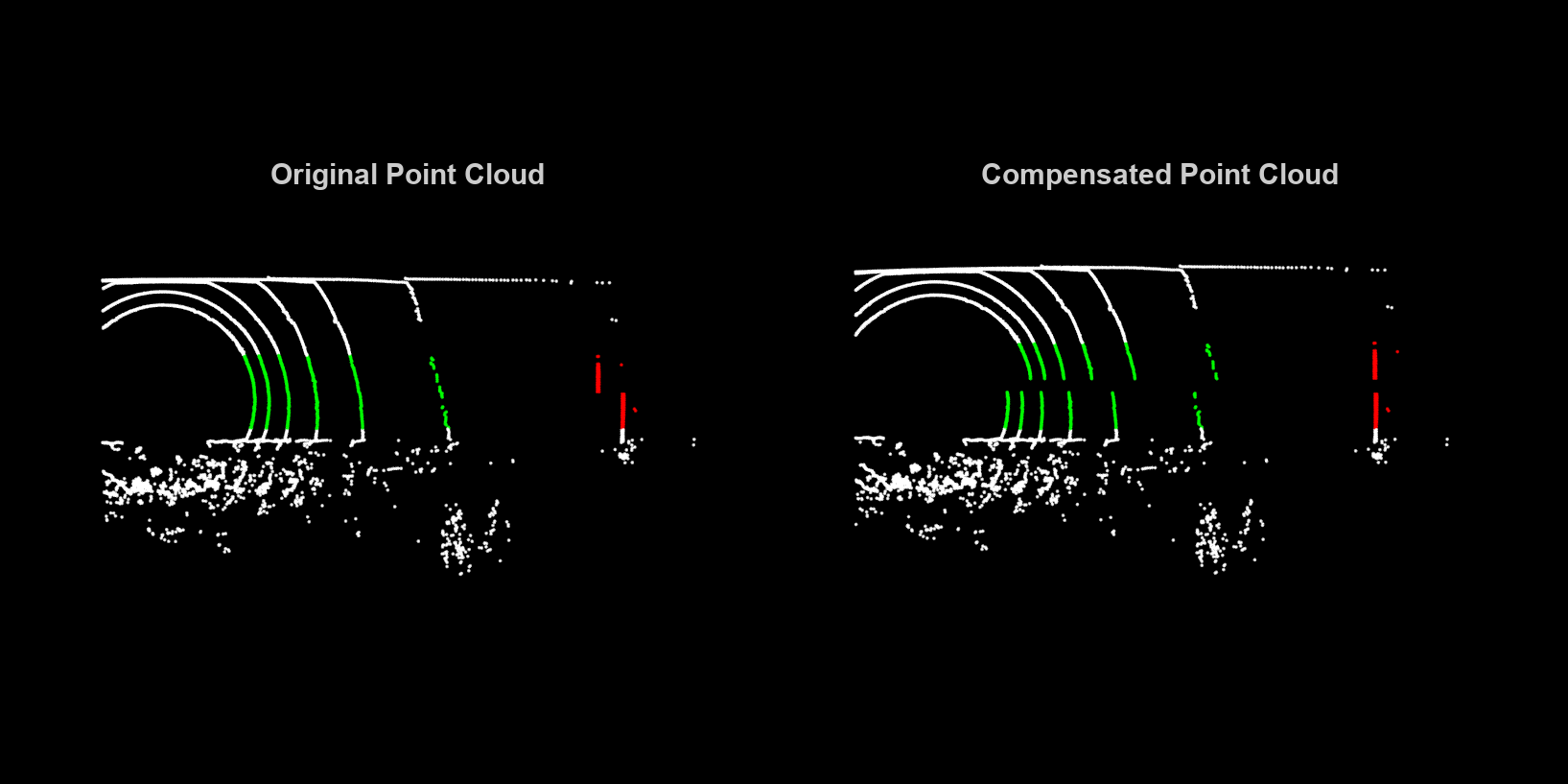
Visualize the effect of the motion compensation on the point cloud data. The green region shows the effect of motion compensation on the ground, and the red region shows the effect of motion compensation on the sign board.

helperVisualizeMotionCompensation(currPtCloud,compensatedPtCloud)

Loop Through Data

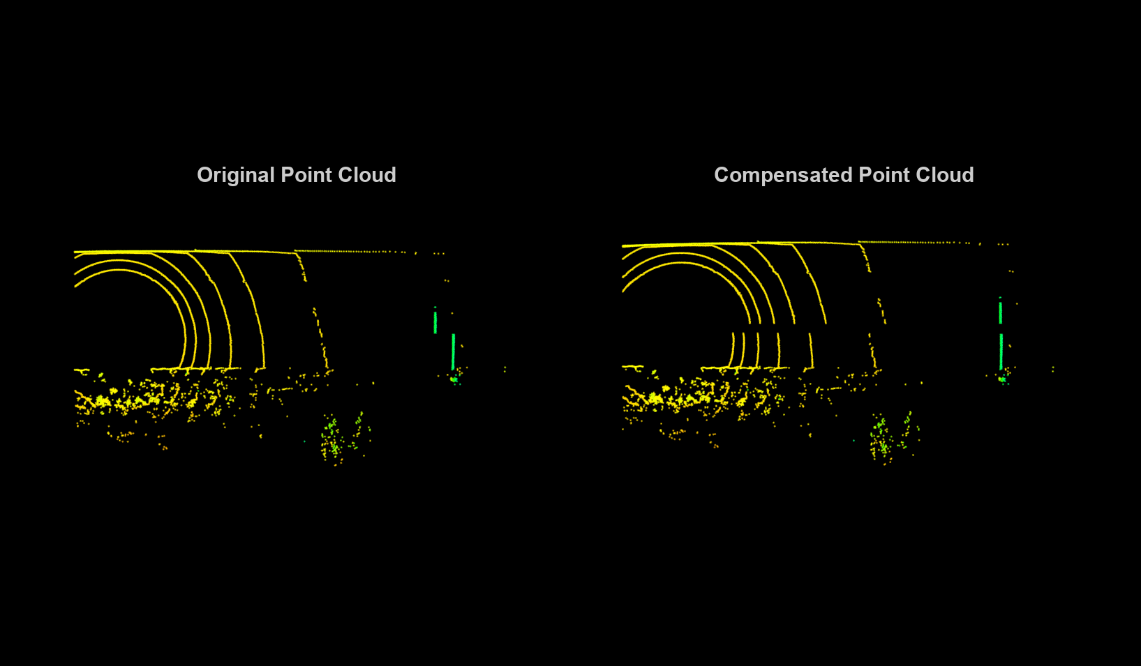
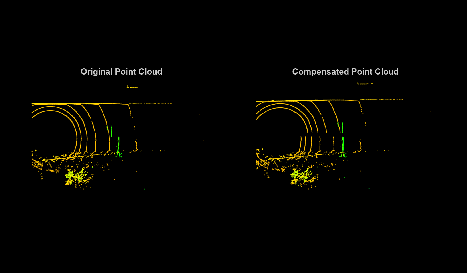
Loop through the selected frames in the recorded lidar data, perform motion compensation, and visualize the compensated point cloud data.

hFigLoop = figure(Position=[0 0 1500 750]);
axCurrPt = subplot(1,2,1,Parent=hFigLoop);
set(axCurrPt,Position=[0.05 0.05 0.42 0.9])
axCompPt = subplot(1,2,2,Parent=hFigLoop);
set(axCompPt,Position=[0.53 0.05 0.42 0.9])

for frameId =  1:numel(lidarDataAlign)
    currPtCloud = lidarDataAlign(frameId);

    % Estimate the timestamp of each point using the organized structure of
    % the point cloud
    [numRows, numColumns, ~] = size(currPtCloud.Location);
    timeFraction = (1:numColumns)/numColumns;
    timeFraction = repmat(timeFraction,numRows,1);
    pointTimestamps = seconds(timeFraction * sweepDuration);

    % Find the relative motion during the lidar sweep
    relTform = rigidtform3d(invert(egoTformLidarENU(frameId+1)).A * egoTformLidarENU(frameId).A);

    % Undistort the point cloud
    compensatedPtCloud = undistortEgoMotion(currPtCloud, relTform, pointTimestamps, sweepTime);

    % Visualize original and compensated point clouds
    pcshow(currPtCloud,Parent=axCurrPt)
    set(axCurrPt,XLim=[-5 45],YLim=[-15 15])
    title(axCurrPt,"Original Point Cloud",FontSize=15)
    colormap(axCurrPt,hsv)
    axis(axCurrPt,'off')
    view(axCurrPt,2)
    pcshow(compensatedPtCloud,Parent=axCompPt)
    set(axCompPt,XLim=[-5 45],YLim=[-15 15])
    title(axCompPt,"Compensated Point Cloud",FontSize=15)
    colormap(axCompPt,hsv)
    axis(axCompPt,'off')
    view(axCompPt,2)
    drawnow("limitrate")
end