Transmit-Receive Chain Processing

Transmit-Receive Chain

This example shows how to implement an LTE transmit and receive chain, as shown in this figure.

Generate an E-UTRA test model (E-TM) configuration. Use this configuration to generate the waveform and populate the resource grid.

enb = lteTestModel('1.1','1.4MHz');
[txwave,txgrid,info] = lteTestModelTool(enb);

Plot a graphical representation of the transmit resource grid.

hPlotDLResourceGrid(enb,txgrid);
title('Transmitted Resource Grid');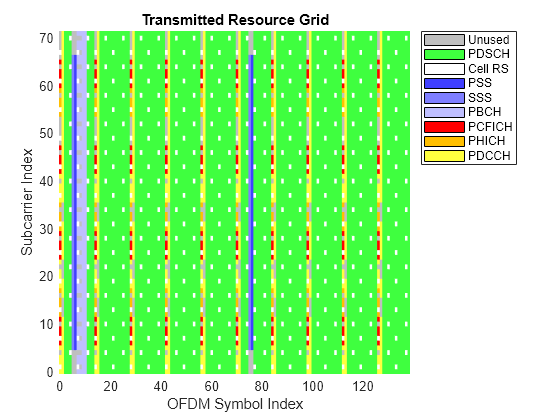

Figure contains an axes object. The axes object with title Transmitted Resource Grid, xlabel OFDM Symbol Index, ylabel Subcarrier Index contains 10 objects of type patch, surface. These objects represent Unused, PDSCH, Cell RS, PSS, SSS, PBCH, PCFICH, PHICH, PDCCH.

The figure shows a resource grid populated with E-TM 1.1 resource elements.

Simulate transmission through a fading channel propagation model.

channel.ModelType = 'GMEDS';
channel.DelayProfile = 'EVA';
channel.DopplerFreq = 70;
channel.MIMOCorrelation = 'Medium';
channel.NRxAnts = 1;
channel.InitTime = 0;
channel.InitPhase = 'Random';
channel.Seed = 17;
channel.NormalizePathGains = 'On';
channel.NormalizeTxAnts = 'On';
channel.SamplingRate = info.SamplingRate;
channel.NTerms = 16;
rxwave = lteFadingChannel(channel,[txwave;zeros(25,1)]);

Plot the time-varying power of the received waveform.

figure('Color','w');
helperPlotReceiveWaveform(info,rxwave);

Figure contains an axes object. The axes object with title Absolute value of received waveform, xlabel Time (s), ylabel Absolute value contains an object of type line.

This plot shows the waveform power variation over time.

Perform frame synchronization.

offset = lteDLFrameOffset(enb,rxwave);
rxwave = rxwave(offset:end,:);

Perform OFDM demodulation.

rxgrid = lteOFDMDemodulate(enb,rxwave);

Create a surface plot showing the power of the received grid for each subcarrier and OFDM symbol.

figure('Color','w');
colors = hIdentifyDLChannels(enb,rxgrid); % Obtain resource grid colorization
hPlotResourceGrid(abs(rxgrid),colors);
title('Received Resource Grid');

Figure contains an axes object. The axes object with title Received Resource Grid, xlabel OFDM symbol index, ylabel Subcarrier index contains an object of type surface.

This plot shows the received grid power.

Estimate the channel and noise.

cec.PilotAverage = 'UserDefined';
cec.FreqWindow = 9;
cec.TimeWindow = 9;
cec.InterpType = 'Cubic';
cec.InterpWindow = 'Centered';
cec.InterpWinSize = 3;
[hest,nest] = lteDLChannelEstimate(enb,cec,rxgrid);

Create a surface plot showing the magnitude of the channel estimate for each OFDM symbol across the subcarriers.

figure('Color','w');
helperPlotChannelEstimate(hest);

Figure contains an axes object. The axes object with title Estimate of channel magnitude frequency response, xlabel OFDM symbol index, ylabel Subcarrier index contains an object of type surface.

This figure shows an estimate of channel magnitude frequency response.

Finally, perform minimum mean-square error (MMSE) equalization on the received grid.

eqgrid = lteEqualizeMMSE(rxgrid,hest,nest);

Create a surface plot of the power of the equalized resource grid, in dB.

figure('Color','w');
colors = hIdentifyDLChannels(enb,eqgrid); % Obtain resource grid colorization
hPlotResourceGrid(abs(eqgrid),colors);
title('Equalized Resource Grid');

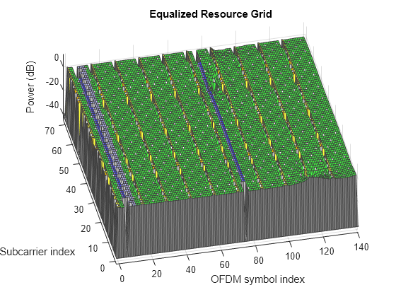
Figure contains an axes object. The axes object with title Equalized Resource Grid, xlabel OFDM symbol index, ylabel Subcarrier index contains an object of type surface.

As can be seen the equalization flattened the power response across the resource grid.