可视化体数据
以下示例演示在 MATLAB® 中以可视方式呈现体数据的几种方法。
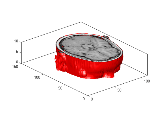
显示等值面
等值面指空间体内的所有点都具有一个常量值的曲面。使用 isosurface 函数生成曲面外的面和顶点,并使用 isocaps 函数生成体端顶的面和顶点。使用 patch 命令绘制空间体及其端顶。
load mri D
D = squeeze(D);
limits = [NaN NaN NaN NaN NaN 10]
limits = 1×6

   NaN   NaN   NaN   NaN   NaN    10
[x, y, z, D] = subvolume(D, limits);
[fo,vo] = isosurface(x,y,z,D,5);
[fe,ve,ce] = isocaps(x,y,z,D,5);
figure
p1 = patch('Faces', fo, 'Vertices', vo);
p1.FaceColor = 'red'
p1 =
  Patch with properties:

    FaceColor: [1 0 0]
    FaceAlpha: 1
    EdgeColor: [0.1294 0.1294 0.1294]
    LineStyle: '-'
        Faces: [23351×3 double]
     Vertices: [12406×3 double]

  Show all properties
p1.EdgeColor = 'none'p1 =
Patch with properties:
FaceColor: [1 0 0]
FaceAlpha: 1
EdgeColor: 'none'
LineStyle: '-'
Faces: [23351×3 double]
Vertices: [12406×3 double]
Show all properties
p2 = patch('Faces', fe, 'Vertices', ve, ...
   'FaceVertexCData', ce)
p2 =
  Patch with properties:

    FaceColor: [0.1294 0.1294 0.1294]
    FaceAlpha: 1
    EdgeColor: [0.1294 0.1294 0.1294]
    LineStyle: '-'
        Faces: [27265×3 double]
     Vertices: [14250×3 double]

  Show all properties
p2.FaceColor = 'interp';
p2.EdgeColor = 'none';

view(-40,24)
daspect([1 1 0.3])
colormap(gray(100))
box on

camlight(40,40)
camlight(-20,-10)
lighting gouraud
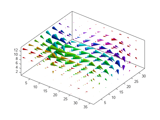
创建锥体绘图
coneplot 命令在空间体的 x、y、z 点处将速度向量绘制为锥体。锥体表示在每个点处向量场的幅值和方向。
cla
load wind u v w x y z
[m,n,p] = size(u)
m =
35
n =
41
p =
15
[Cx, Cy, Cz] = meshgrid(1:4:m,1:4:n,1:4:p);
h = coneplot(u,v,w,Cx,Cy,Cz,y,4);
set(h,'EdgeColor', 'none')

axis tight equal
view(37,32)
box on
colormap(hsv)
light
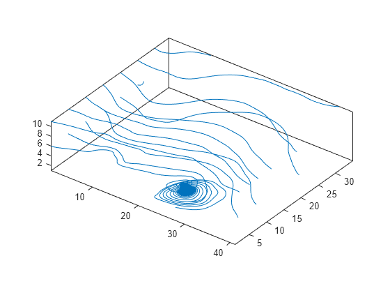
绘制流线图
streamline 函数在空间体的 x、y、z 点处绘制速度向量的流线图,以表示三维向量场的流向。
cla

[m,n,p] = size(u);
[Sx, Sy, Sz] = meshgrid(1,1:5:n,1:5:p);
streamline(u,v,w,Sx,Sy,Sz)

axis tight equal
view(37,32)
box on
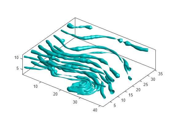
绘制流管图
streamtube 函数在空间体的 x、y、z 点处将速度向量绘制为流管图。管的宽度与每个点处向量场的归一化发散成比例。
cla

[~,n,p] = size(u);
[Sx, Sy, Sz] = meshgrid(1,1:5:n,1:5:p);
h = streamtube(u,v,w,Sx,Sy,Sz);
set(h, 'FaceColor', 'cyan')
set(h, 'EdgeColor', 'none')

axis tight equal
view(37,32)
box on
light
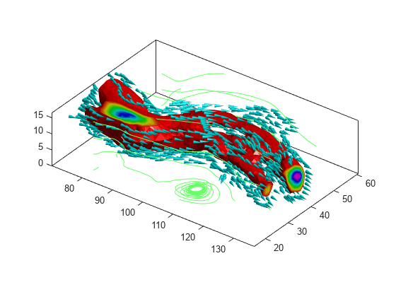
合并不同空间体的可视化绘图
在单个绘图中合并空间体的可视化绘图以生成更为全面的体内速度场全貌。
cla
spd = sqrt(u.*u + v.*v + w.*w);
[fo,vo] = isosurface(x,y,z,spd,40);
[fe,ve,ce] = isocaps(x,y,z,spd,40);
p1 = patch('Faces', fo, 'Vertices', vo);
p1.FaceColor = 'red'
p1 =
  Patch with properties:

    FaceColor: [1 0 0]
    FaceAlpha: 1
    EdgeColor: [0.1294 0.1294 0.1294]
    LineStyle: '-'
        Faces: [5340×3 double]
     Vertices: [2727×3 double]

  Show all properties
p1.EdgeColor = 'none'p1 =
Patch with properties:
FaceColor: [1 0 0]
FaceAlpha: 1
EdgeColor: 'none'
LineStyle: '-'
Faces: [5340×3 double]
Vertices: [2727×3 double]
Show all properties
p2 = patch('Faces', fe, 'Vertices', ve, ...
   'FaceVertexCData', ce)
p2 =
  Patch with properties:

    FaceColor: [0.1294 0.1294 0.1294]
    FaceAlpha: 1
    EdgeColor: [0.1294 0.1294 0.1294]
    LineStyle: '-'
        Faces: [464×3 double]
     Vertices: [301×3 double]

  Show all properties
p2.FaceColor = 'interp'p2 =
Patch with properties:
FaceColor: 'interp'
FaceAlpha: 1
EdgeColor: [0.1294 0.1294 0.1294]
LineStyle: '-'
Faces: [464×3 double]
Vertices: [301×3 double]
Show all properties
p2.EdgeColor = 'none' p2 =
Patch with properties:
FaceColor: 'interp'
FaceAlpha: 1
EdgeColor: 'none'
LineStyle: '-'
Faces: [464×3 double]
Vertices: [301×3 double]
Show all properties
[fc, vc] = isosurface(x, y, z, spd, 30);
[fc, vc] = reducepatch(fc, vc, 0.2);
h1 = coneplot(x,y,z,u,v,w,vc(:,1),vc(:,2),vc(:,3),3);
h1.FaceColor = 'cyan';
h1.EdgeColor = 'none';

[sx, sy, sz] = meshgrid(80, 20:10:50, 0:5:15);
h2 = streamline(x,y,z,u,v,w,sx,sy,sz);
set(h2, 'Color', [.4 1 .4])

axis tight equal
view(37,32)
box on
light