Export Models to the Workspace
Export Models to MATLAB
You can export models to the workspace to work with them in MATLAB®.
From the Model Browser test plan or any model node, select File > Export Models. The Export Models dialog box opens.
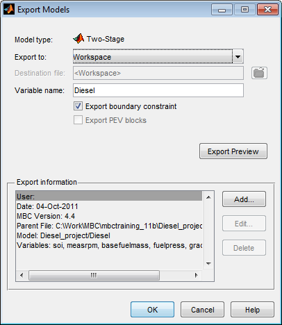
Select
Workspacefrom the Export to list.Edit the Variable name if desired.
If you have a boundary constraint, it is exported unless you clear the Export boundary constraint check box.
(Optional) Click Export Preview to check the models you selected for export:
From the test plan node, you export all the response models in the test plan (provided you have selected best models for them all), or point-by-point models (when all local models are multiple models).
From a local model, you export all the local models as a point-by-point model.
From other model nodes, you export only the current model.
The Model type field on the Export Models dialog box displays the type of model you are exporting: two-stage, point-by-point, or other model type.
(Optional) Click Add to add a comment to Export information.
Click OK to export the models to the workspace.
Work with Models in the Workspace
After exporting the model to the workspace, you can:
Evaluate the model.
Evaluate the prediction error variance (PEV).
Evaluate the boundary model.
Calculate confidence intervals for model prediction.
Exported models appear in your workspace as an
xregstatsmodel or mbcPointByPointModel object,
or a cell array of models. You use the same commands to evaluate
xregstatsmodel or mbcPointByPointModel
models.
If you export a group of models, the toolbox exports a cell array of models. The
argument order in the cell array {1 to n} corresponds to the top-down
model order in the model tree in the Model Browser.
Evaluate Response Models and PEV
For example, if you export a model to the workspace as MyModel and
the model has four input factors, evaluate the model at a point as shown here:
Y = MyModel([3.7,89.55,-0.005,1]);
If you create column vectors
p1,p2,p3,p4
(of equal length) for each input factor, you can evaluate the model to give a column vector
output:
Y = MyModel([p1,p2,p3,p4]);
Left-to-right argument order corresponds to the top-down input order in the Test Plan view in the Model Browser.
The inputs and outputs for MATLAB model evaluation are in natural engineering units, not coded units.
You can evaluate the PEV for the model using the command:
[pev, y] = pev(MyModel, [x1 x2 x3])
You can use one or two arguments, as follows:
[p] = pev(x) gives pev at
x.
[p,y] = pev(x) gives pev at x
and model evaluation at x.
For more information, see xregstatsmodel.
Evaluate Confidence Intervals
Use predint to evaluate the model confidence intervals:
Interval = predint(StatsModel,X,Level);
Level
confidence interval of the predictions is calculated about the predicted value. The default
value for Level is 99. Interval is
an Nx2 array where the first column is the lower bound and the second
column is the upper bound.The confidence interval is given by:
upperbound = y + t*sqrt(pev)
lowerbound = y - t*sqrt(pev)
where y is the model prediction, and t is the
appropriate percentile of the t-statistic, with df = nObs–1 degrees of freedom. The toolbox
calculates this using the Statistics and Machine Learning Toolbox™ function tinv as follows:
t = tinv(p,v)
p = confidence level, e.g., 95%
v = degrees of freedom (n-1)
t = tinv(1-alpha/2, df)
where alpha = 0.05 for 95% confidence intervals.
Evaluate Boundary Models in the Workspace
You can use the function ceval to evaluate a boundary constraint
exported to the workspace. For example, if your exported model is M, then
ceval(M, X)
M at the points given by the matrix X. Values less
than 0 are inside the boundary. See Explore Boundary Model Types.For example, if you exported multiple responses from a test plan as a cell array named
modeltutorial, entering the following at the command line evaluates the
boundary model for the first response {1} at the point where all four inputs are 0:
ceval(modeltutorial{1}, [0,0,0,0])
Response models are in top-down order in the model tree. For example, {1} is the top model in the tree under the test plan node. [0,0,0,0] is the matrix of input values, where left-to-right argument order corresponds to the top-down input order in the Boundary Editor or the Test Plan view in the Model Browser, e.g., spk, load, rpm, and afr.
You can quickly check the number of model inputs as follows:
nfactors(modeltutorial{1})
You can click a point in the boundary editor (in the 1-D, 2-D, and 3-D views) to check the input names and get example input values to evaluate in the workspace, e.g.,
ceval (modeltutorial{1},[25, 0.64, 5000, 14.43])
ans = 3.0284e-004
Boundary constraint distance of 0 means the point is on the boundary, negative values are inside the constraint, and positive values are outside. The range is typically [–1,1] but not always, and roughly linear. Rather like information criteria, it is only a comparison that is meaningful (point x has a greater distance than point y) rather than the absolute value.
For more information, see xregstatsmodel.