Design and Simulate Resonant Converter Control

Direct Frequency Control

Direct Frequency Control varies the switching frequency $$F_{sw}$$ directly through the PI controller output. Higher $$F_{sw}$$ moves operation further above resonance and reduces $$V_{out}$$. Lower $$F_{sw}$$ moves operation closer to resonance and increases $$V_{out}$$. DFC is the classical LLC control strategy and works over a wide power range.

To open the prebuilt DFC model, use open_system. The model loads the DFC plant and controller parameters using the DFC data script. This script calls getResonantConverterParam('Converter100W') to load a 400 V input, 54 V output, 100 W half-bridge preset, then sets TsVolt = 50 µs, TsPlant = 1/50e6, VRef = ResonantConv.Vout, and the open-loop switching frequency FswOpen = 1.2 * ResonantConv.Fres.

open_system("LLCVoltageControlWithDFC")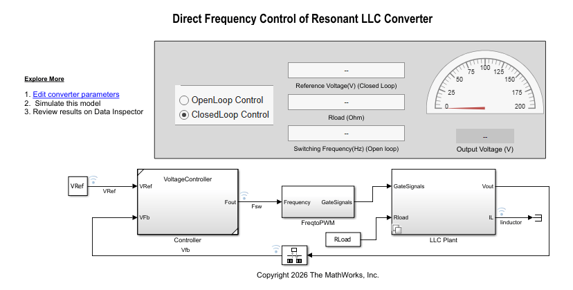

The model contains a variant LLC Plant subsystem and a Controller subsystem. The Controller subsystem pairs a Resonant Converter Gains block with a Resonant Voltage Controller block. Both blocks come from the Power Converter Control with Motor Control Blockset™ library. The Resonant Converter Gains block derives the PI gains internally from the converter dialog values and passed to the Resonant Voltage Controller at run time. No manual tuning is needed. The LoopSelect block selects open-loop or closed-loop operation. Set it to 0 to inject the fixed frequency FswOpen, or 1 to close the loop with the PI controller.

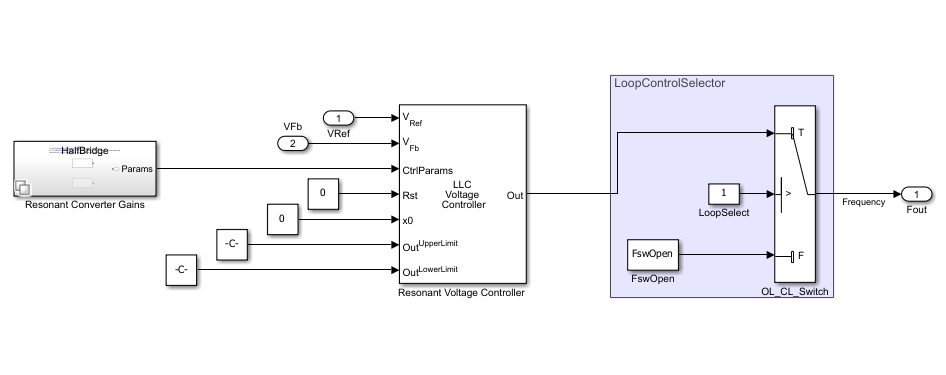
Run the closed-loop simulation.

set_param("LLCVoltageControlWithDFC/Controller/LoopSelect", Value="1")  % Close the loop
sim("LLCVoltageControlWithDFC");
dfcRunIDs = Simulink.sdi.getAllRunIDs();
dfcRun = Simulink.sdi.getRun(dfcRunIDs(end));  % Get the most recent simulation run
dfcVfb = dfcRun.getSignal(dfcRun.getSignalIDsByName("Vfb")).Values;  % Output voltage feedback
dfcFsw = dfcRun.getSignal(dfcRun.getSignalIDsByName("Fsw")).Values;  % Commanded switching frequency

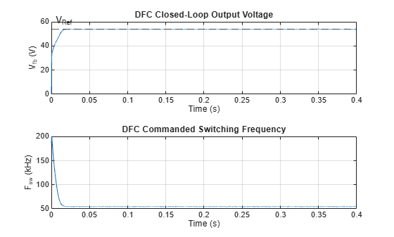
To visualize the closed-loop DFC response, plot the output voltage and the commanded switching frequency on separate axes. The controller drives $$V_{fb}$$ toward $$V_{Ref}$$. The switching frequency settles at the value required to hold the output at the reference under nominal load. The trade-off is that the switching frequency varies with load and line conditions. As a result, magnetics and EMI filters must be designed to accommodate the full frequency range [FswMin, FswMax] from the converter preset.

figure
t = tiledlayout(2,1);
nexttile  % Top tile: output voltage vs. reference
plot(dfcVfb.Time, dfcVfb.Data)
yline(VRef, "--", "V_{Ref}", LabelHorizontalAlignment="left")
xlabel("Time (s)")
ylabel("V_{fb} (V)")
title("DFC Closed-Loop Output Voltage")
grid on

nexttile  % Bottom tile: switching frequency adapts to regulate voltage
plot(dfcFsw.Time, dfcFsw.Data / 1e3)
xlabel("Time (s)")
ylabel("F_{sw} (kHz)")
title("DFC Commanded Switching Frequency")
grid on

Select Parameters for Time-Shift Control

Time-Shift Control keeps the switching cadence fixed and modulates $$T_D$$ instead.

The first step is to select the plant parameters. The getResonantConverterParam function provides three presets:

ConverterParam = 'Converter100W';  % Choose a preset
ResonantConv = getResonantConverterParam(ConverterParam);  % Returns struct with Vin, Vout, Pout, Fres, FswMin, FswMax, etc.
RLoad = ResonantConv.Vout^2/ResonantConv.Pout;  % Nominal load resistance (Ohms)

Select the switching topology of the LLC power stage. The preset returns HalfBridge by default. Switch to FullBridge to select the full-bridge variant of the plant.

PlantConfig = ResonantConv.PlantConfig;  % 'HalfBridge' by default; override to 'FullBridge' if needed

Set the sample times for the discrete-time controller implementation. The voltage loop runs at 50 µs, and the plant simulation step matches the 50 MHz FPGA clock.

TsVolt  = 50e-6;      % Voltage control loop sample time (50 µs)
FFpga   = 50e6;       % FPGA clock frequency (50 MHz)
TsPlant = 1/FFpga;    % Plant simulation step size matches FPGA clock

Set the target output voltage for closed-loop regulation.

VRef = ResonantConv.Vout;  % Target output voltage for closed-loop regulation

Compute the $$T_D$$ limits and switch dead-time in FPGA clock counts for use in the modulator.

TD_min       = 1/(4*ResonantConv.FswMax);       % Minimum TD: largest power transfer (highest Fsw)
TD_max       = 1/(2.5*ResonantConv.FswMin);     % Maximum TD: smallest power transfer (lowest Fsw)
Tdead        = ResonantConv.Tdead;              % Switch dead-time (s)
Tdead_counts = uint32(Tdead / TsPlant);         % Dead-time in FPGA clock counts

Set the startup $$T_D$$ to TD_max so the converter starts in a low-power state and the output ramps up smoothly. Initialize the PI gains to small placeholder values so the model can compile during the open-loop identification runs. The placeholders are inactive when LoopSelect is 0 and are replaced with the designed values before the closed-loop simulation.

TD_initial = TD_max;   % Start at maximum TD for a smooth low-power startup ramp
Kp_TSC = 1e-10;        % Placeholder Kp
Ki_TSC = 1e-8;         % Placeholder Ki

Add the Utilities folder to the path so the helper functions used below are visible.

addpath(fullfile(pwd, 'Utilities')); 

Run Open-Loop Simulations to Identify the Plant

To design a controller, you must first understand how the plant responds. In TSC control, the "plant" is the mapping from $$T_D$$ to output voltage $$V_{out}$$.

Identify the plant by running open-loop simulations at different equally-spaced $$T_D$$ values between $$T_{D,min}$$ and $$T_{D,max}$$. In each simulation, the controller is disconnected (open-loop mode) and a constant $$T_D$$ is applied. The output voltage $$V_{fb}$$ rises from zero and settles to a steady-state value that depends on the applied $$T_D$$. For simulation, use the same TSC model that operates in open loop as well as in closed loop.

ModelName = 'LLCVoltageControlWithTSC';
open_system(ModelName)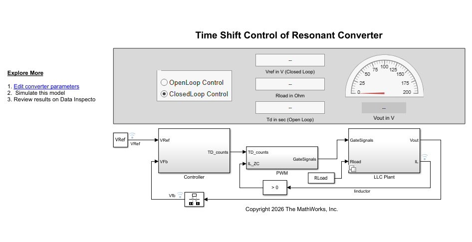

From each response, extract:

n = 5;           % Number of equally-spaced TD operating points to sweep
simTime = '0.01';
openloopresult = simulateOpenLoop(ModelName, TD_min, TD_max, n, simTime);  % Returns Vss and tau per operating point

Warning: Graphics acceleration hardware is unavailable. Graphics quality and performance might be diminished. See <a href="https://www.mathworks.com/support/requirements/matlab-system-requirements.html">MATLAB System Requirements</a>.

The plot below shows the output voltage versus time for each of the $$T_D$$ values. Key observations:

clf
figure
plotOpenLoopResponses(openloopresult);  % Vout vs. time for each TD: lower TD → higher steady-state voltage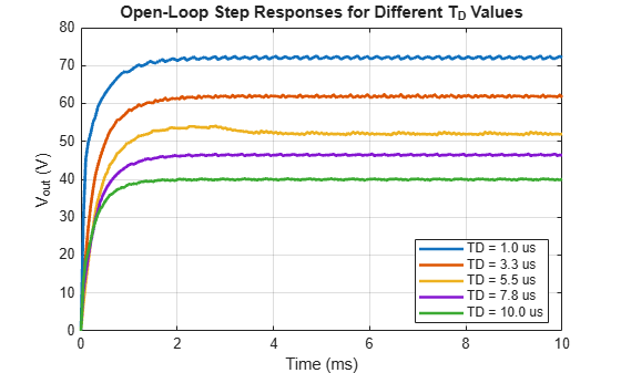

By normalizing each response to its own steady-state value, you can visually verify that the dynamics (time constant) are consistent across different operating points. If all curves overlap, the first-order linear model is a good approximation across the operating range.

clf
figure
plotNormalizedResponses(openloopresult);  % Overlapping curves confirm consistent first-order dynamics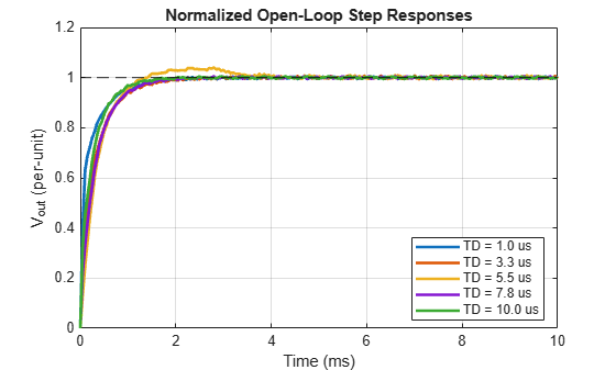

Fit the First-Order Plant Model

Model the plant as a first-order transfer function $$G(s)=K/(\tau s+1)$$, where $$K$$ is the plant DC gain in V/s (the slope of a linear regression of $$V_{out,ss}$$ versus $$T_D$$) and $$\tau$$ is the plant time constant in seconds (the average of the individual time-constant fits from all trials). A negative value of $$K$$ indicates that increasing $$T_D$$ decreases $$V_{out}$$, which is the expected control direction for TSC.

[K, tau] = fitPlantModel(openloopresult)  % K: DC gain (V/s, negative); tau: time constant (s)

K = 
-3.5439e+06

tau = 
3.3678e-04

Design the PI Controller by Pole-Zero Cancellation

The closed-loop control system consists of:

The open-loop transfer function is $$L(s)=C(s)\cdot G(s)\cdot H(s)$$. The key design is by choosing $$K_i/K_p=1/\tau$$, the PI controller's zero exactly cancels the plant's pole. This simplifies the open-loop to a pure integrator $$L(s)=\frac{|K|\cdot K_p}{\tau \cdot s}$$. A pure integrator has exactly 90° phase margin at any crossover frequency. This guarantees a stable, overdamped closed-loop response with no oscillations.

The crossover frequency $${\omega }_c$$ determines how fast the closed-loop responds to disturbances and reference changes. Choose $${\omega }_c$$ based on:

Increasing $${\omega }_c$$ gives faster disturbance rejection but reduces phase margin and robustness. The rule of thumb is to keep $${\omega }_c\ll 1/\tau$$ for the pole-zero cancellation to yield an overdamped response.

wc = 0.2; 

From the unity-gain crossover condition $$|L(j{\omega }_c)|=1$$, compute $$K_p=\tau {\omega }_c/|K|$$ and $$K_i=K_p/\tau$$. The verification struct returned by computePIGains reports the actual loop gain magnitude and phase margin at $${\omega }_c$$.

[Kp_TSC, Ki_TSC, verification] = computePIGains(K, tau, TsVolt, wc)

Kp_TSC = 
1.9006e-11

Ki_TSC = 
5.6435e-08

verification = struct with fields:
          mag_at_wc: 1.0000
    phase_at_wc_deg: -90.0003
          PM_actual: 89.9997

The verification confirms $$|L(j{\omega }_c)|\approx 1$$ (unity gain at crossover) and phase margin $$\approx 90°$$ (overdamped, no oscillation).

Simulate the Closed-Loop System

With the PI gains computed, close the loop and simulate the full system. The controller uses the computed $$K_p$$ and $$K_i$$ to regulate $$V_{fb}$$ to track the reference voltage $$V_{Ref}$$. Expect:

simTime = '0.01';  % 10 ms simulation; enough for Vout to settle to VRef
closedloopresult = simulateClosedLoop(ModelName, Kp_TSC, Ki_TSC, simTime);  % Assigns Kp_TSC/Ki_TSC to base workspace, closes loop, runs sim

Plot the closed-loop response. The controller drives $$V_{fb}$$ toward $$V_{Ref}$$ with an overdamped shape and no overshoot, consistent with the 90° phase margin design.

clf
figure
plotClosedLoopResponse(closedloopresult);  % Vfb rises to VRef with overdamped shape and no overshoot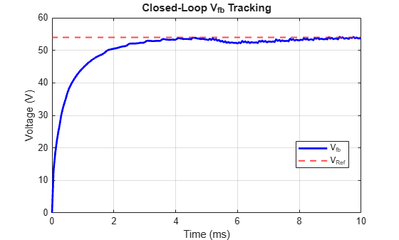

You simulated voltage regulation for an LLC resonant converter under two different modulation strategies. Direct Frequency Control adjusts $$F_{sw}$$ directly through a PI controller. The gains are auto-computed from the plant dialog values on the Resonant Converter Gains block. DFC is a good default when the resulting frequency range is acceptable for the magnetics and EMI filter design. Time-Shift Control keeps the switching cadence fixed and modulates $$T_D$$ instead. The $$T_D$$-to-$$V_{out}$$ plant is approximately first-order. An open-loop system-identification workflow paired with pole-zero cancellation delivers a PI controller with 90° phase margin.

To adapt this workflow to a new LLC plant, change ConverterParam to another preset from getResonantConverterParam (or add a new preset), then rerun the identification and design sections. The utility functions compute new gains. Precomputed reference gains for the three shipped presets are stored in LLCVoltageControlWithTSCData.m so you can jump straight to closed-loop simulation for those presets. To try a different power-stage topology, override PlantConfig to 'FullBridge' before opening the model. Both harness models switch between half-bridge and full-bridge automatically. Reference standalone plants are provided in HalfBridgeLLCConverter.slx and FullBridgeLLCConverter.slx.