Design and Simulate Boost PFC Controllers

Load Parameters and Open the Model

Open the prebuilt SimulateBoostPFC harness model to inspect the control architecture before running the simulation.

open_system("SimulateBoostPFC")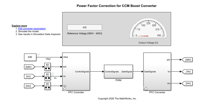

The model contains a PFC Converter subsystem, a PFC Controller subsystem, and a PWM subsystem. The PFC Controller subsystem implements a cascaded structure: a CalculateControllerGains subsystem that uses the PFC Controller Gains block to compute proportional-integral (PI) gains from converter parameters and the sample times, a VoltageController subsystem with anti-windup clamping and a rate limiter for soft-start, and a CurrentController subsystem with a second-order generalized integrator phase-locked loop (SOGI-PLL) for in-phase current shaping.

The SimulateBoostPFC model uses Simulink(R) variant subsystems to switch between the classical and totem-pole boost PFC topologies. The workspace variable PFCConfig controls which variant is active. Set PFCConfig to 'Classical' to activate the classical full-bridge diode rectifier with a single N-channel MOSFET boost switch.

PFCConfig = 'Classical';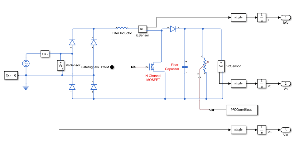

Run BoostPFCSimData to load topology-specific plant parameters and compute sample times. The script calls PFCPlantParameters(PFCConfig) to populate the struct PFCConv with values for the classical topology: a 50 kHz switching frequency, 1.9 mH boost inductor, 748 µF output capacitor, and 200 Ω load for 1000 W at 400 V DC from a 120 Vrms, 60 Hz input. The script also sets Ts (20 µs current-loop sample time), TsVolt (200 µs voltage-loop sample time, 10× Ts), and TsPlant (plant simulation step, 1/50 of the switching period).

BoostPFCSimData;

Simulate the Classical Boost PFC Converter

With plant parameters loaded, simulate the classical topology to verify closed-loop output voltage regulation and current controller performance. Pass 0.6 as the stop time. Both topologies settle to steady state within 0.6 s. This time captures the full start-up transient and several line cycles at steady state.

simOut = sim("SimulateBoostPFC", 0.6);

Retrieve the logged signals from the Simulation Data Inspector (SDI). The call to getAllRunIDs returns all run identifiers in the current session. The index runIDs(end) selects the most recent run, which corresponds to the simulation you just ran.

runIDs = Simulink.sdi.getAllRunIDs();
pfcRunCL = Simulink.sdi.getRun(runIDs(end));

Retrieve output voltage, inductor current feedback, and peak current reference amplitude by signal name. Vo is the output voltage, Ifb_IControl is the inductor current feedback, and IRef_IControl is the peak current reference amplitude produced by the voltage controller.

voDataCL   = pfcRunCL.getSignal(pfcRunCL.getSignalIDsByName("Vo")).Values;
ifbDataCL  = pfcRunCL.getSignal(pfcRunCL.getSignalIDsByName("Ifb_IControl")).Values;
irefDataCL = pfcRunCL.getSignal(pfcRunCL.getSignalIDsByName("IRef_IControl")).Values;

Examine Output Voltage Regulation

Plot the output voltage over the full 0.6 s simulation to verify that the voltage controller ramps the output to the 400 V reference and holds it in steady state. The rate limiter in the VoltageController subsystem prevents an inrush current surge during start-up by limiting the rate at which the reference ramp rises.

figure
plot(voDataCL.Time, voDataCL.Data)
yline(400, "--r", "V_{ref} = 400 V")
xlabel("Time (s)")
ylabel("Output Voltage (V)")
title("Classical Boost PFC — Output Voltage")

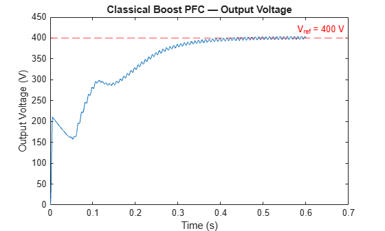
The output voltage ramps from 0 V and settles to approximately 400 V before 0.6 s, confirming that the voltage loop PI gains computed by the PFC Controller Gains block provide stable regulation. The dashed reference line at 400 V shows that steady-state error is negligible.

Examine Inductor Current Waveform

Examine the inductor current over the last two AC line cycles to assess current shaping quality at steady state. PFCConv.FRated holds the rated line frequency (60 Hz for the classical topology), so 2/PFCConv.FRated spans exactly two line cycles. Restricting the plot window to steady state removes the start-up transient and focuses on the sinusoidal envelope that indicates unity power factor operation.

tStart = 0.6 - 2/PFCConv.FRated;
tMask = ifbDataCL.Time >= tStart;

IRef_IControl is a scalar peak amplitude produced by the outer voltage controller. It represents the desired peak of the inductor current envelope, not a time-varying sinusoid. Use max(irefDataCL.Data) to extract the settled peak amplitude and display it as a horizontal reference on the plot.

irefPeakCL = max(irefDataCL.Data);

figure
plot(ifbDataCL.Time(tMask), ifbDataCL.Data(tMask))
yline(irefPeakCL, "--r", ...
    sprintf("I_{ref} peak = %.1f A", irefPeakCL))
xlabel("Time (s)")
ylabel("Inductor Current (A)")
title("Classical Boost PFC — Inductor Current (Last 2 Line Cycles)")

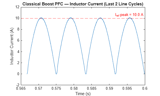
The inductor current tracks a sinusoidal envelope that is in phase with the rectified input voltage, indicating that the SOGI-PLL correctly estimates the AC source phase and frequency. The dashed reference line shows that the current controller drives the peak current to approximately 10 A, matching IRef_IControl produced by the voltage loop.

Simulate the Totem-Pole Boost PFC Converter

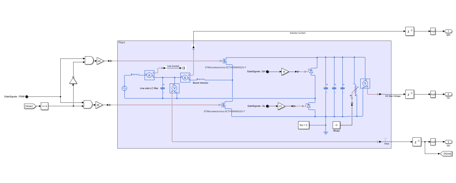
Switch to the totem-pole topology to compare its performance under 230 Vrms, 50 Hz line conditions. Set PFCConfig to 'Totempole' and reload BoostPFCSimData. The data script detects the new value of PFCConfig, calls PFCPlantParameters('Totempole'), and updates PFCConv with the totem-pole plant values: a 72 kHz switching frequency, 0.4 mH boost inductor, 680 µF output capacitor, and 300 Ω load for 1000 W at 400 V DC. It also updates Ts to approximately 13.9 µs and TsVolt to approximately 139 µs.

PFCConfig = 'Totempole';
BoostPFCSimData;

The totem-pole topology replaces the full-bridge diode rectifier with two high-frequency MOSFETs and two line-frequency thyristors. The ThyristorControl subsystem manages commutation of the thyristors at the line frequency to enable bidirectional current flow. Simulate the totem-pole topology for 0.6 s using the same stop time as the classical topology to keep the comparison consistent.

simOut = sim("SimulateBoostPFC", 0.6);

Retrieve the output voltage signal for the totem-pole run from SDI by name. The runIDs(end) index selects the most recent run, which now corresponds to the totem-pole simulation. The totem-pole run logs a different set of signals than the classical run, so retrieve Vo by name rather than index.

runIDs = Simulink.sdi.getAllRunIDs();
pfcRunTP = Simulink.sdi.getRun(runIDs(end));
voDataTP = pfcRunTP.getSignal(pfcRunTP.getSignalIDsByName("Vo")).Values;

Compare Topology Responses

Overlay the output voltage transients for both topologies on a single plot to compare start-up dynamics and steady-state regulation. Both simulations share the same 400 V reference and 1000 W output power target, so any differences in the transient reflect the effect of topology, switching frequency, and filter component values on closed-loop bandwidth.

figure
plot(voDataCL.Time, voDataCL.Data, DisplayName="Classical (120 Vrms, 60 Hz)")
hold on
plot(voDataTP.Time, voDataTP.Data, DisplayName="Totem-pole (230 Vrms, 50 Hz)")
yline(400, "--k", "V_{ref} = 400 V", HandleVisibility="off")
hold off
xlabel("Time (s)")
ylabel("Output Voltage (V)")
title("Boost PFC Topologies — Output Voltage Comparison")
legend(Location="southeast")

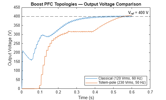
Both topologies settle to approximately 400 V within 0.6 s, confirming that the PFC Controller Gains block computes appropriate PI gains for each set of plant parameters without manual tuning. The totem-pole topology operates at a higher switching frequency with a smaller boost inductor, which changes the current-loop bandwidth and may produce a different transient shape during start-up.

The cascaded control structure has three stages: gain calculation, voltage loop, and current loop. This structure adapts to each topology automatically when you change PFCConfig and reload BoostPFCSimData. To explore further, vary Rload in PFCPlantParameters to test load-step rejection. You can also use the Simulation Data Inspector to examine the duty cycle and voltage feedback signals logged at indices 6 and 5, respectively.