Estimate Lung Displacement Field During Breathing Using Deformable Image Registration

Open Live Script

This example uses deformable image registration to estimate the displacement field between two CT scans acquired during inhalation and exhalation for the same patient.

Deformable image registration aligns 3-D volumes while accounting for non-rigid motion, such as expanding and contracting lung tissue. Deformable registration of CT scans acquired during inhalation and exhalation can map the displacement of lung tissue during the two phases of breathing. Quantifying lung motion is useful for applications such as radiotherapy planning for lung cancer, because precisely targeting treatment can help to avoid damaging healthy tissue.

Download Data

This example uses a subset of data from one subject in a data set containing CT and PET images [1][2]. The subset includes one CT scan acquired during inhalation and one CT scan acquired during exhalation. The size of the subset of data is approximately 137 MB. Run this code to download the data set from the MathWorks® website, and then unzip the folder.

zipFile = matlab.internal.examples.downloadSupportFile("medical", ...
    "CT-PET-Ventilation-Imaging/Chest-Ventilation-Imaging.zip");
filepath = fileparts(zipFile);
unzip(zipFile,filepath)

After you run the code to download the data, the dataFolder folder contains the downloaded and unzipped data. Each scan consists of a directory of DICOM files.

dataFolder = fullfile(filepath,"Chest-Ventilation-Imaging");

Import Data

Read the CT volume acquired at 80% of maximum inhalation as a medicalVolume object.

medVolInsp = medicalVolume(fullfile(dataFolder,"5.000000-Thorax Insp  2.0  B70f-84301"));

Read the CT volume acquired at peak exhalation as a medicalVolume object.

medVolExsp = medicalVolume(fullfile(dataFolder,"7.000000-Thorax Exp  2.0  B70f-98860"));

Display Unregistered Volumes

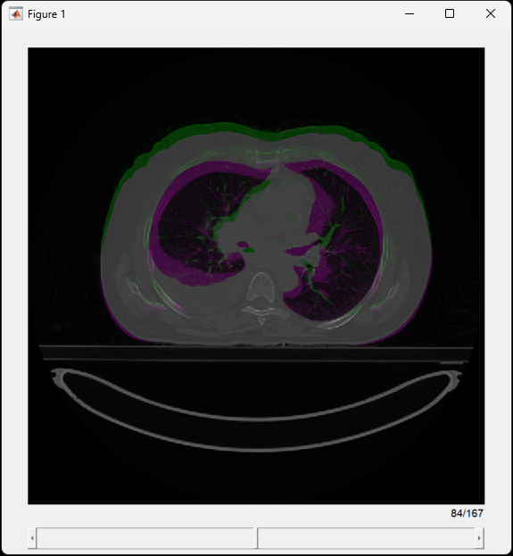
To visualize differences within the lungs, create a falsecolor overlay of the CT volumes by using the displayFusedSlices helper function, defined at the end of this example.

displayFusedSlices(medVolInsp,medVolExsp)

This image shows the middle transverse slice. Purple and green indicate where the images are different. In the inhalation image, the anterior wall of the abdomen is extended and the lung cavity is larger as compared to the exhalation image.

Scrollable sliceViewer window showing the transverse slices of a fused overlay of the unregistered volumes.

Calculate Deformable Registration

Register the CT volume at inhalation to the CT volume at exhalation by using the imregdeform function. The registration can take several minutes. The name-value arguments specified in this example have been determined for this data set by using trial and error.

moving = medVolInsp.Voxels;
fixed = medVolExsp.Voxels;

[dispField,reg] = imregdeform(moving,fixed,PixelResolution=medVolInsp.VoxelSpacing, ...
    NumPyramidLevels=6,GridRegularization=0.01);

--------------------------- Pyramid Level = 6 -------------------------------- 
               Normalized     Function local                          Closeness to
 Iteration        rmse            minima          Step-size        optimal solution
     1          1.62481       39852990.50          14.24              5685.85944
     2          1.62183       38583968.52          37.41              3963.36302
     3          1.62707       36918008.24         142.41              6034.82919
     4          1.61063       35500788.44          55.79              5876.61545
     5          1.62511       34369435.01          73.64              8360.93571
     6          1.60027       33748504.42          30.29              4118.84221
     7          1.58207       33258484.20          37.79              5999.56215
     8          1.57513       32963564.36          23.75              5731.53510
     9          1.58490       32651994.46          63.44              9566.42583
    10          1.58375       32388652.65          27.98              4869.31721
    11          1.57107       32194121.93          29.89              2920.65547
    12          1.57197       32011187.89          78.36             10958.16473
    13          1.57276       31927547.62          46.60              8055.35878
    14          1.56669       31772759.29          21.18              4067.68143
    15          1.55234       31691226.84          41.83              3398.35486
    16          1.54753       31562509.85          24.18              3955.47316

--------------------------- Pyramid Level = 5 -------------------------------- 
               Normalized     Function local                          Closeness to
 Iteration        rmse            minima          Step-size        optimal solution
     1          0.91176       42907652.78           7.65              7088.24860
     2          0.89018       41640846.07          64.12              4231.25487
     3          0.88098       41268677.48          23.56              2308.48118
     4          0.88108       40420137.71          69.98              3017.36869
     5          0.88136       39708273.80          94.18              3004.63424
     6          0.86391       39287029.08          53.18              2836.02841
     7          0.85912       38752913.15          81.04              2839.52290
     8          0.85921       38451159.94          72.15              3121.08355
     9          0.85602       38316538.90          91.19              2466.11900
    10          0.84566       38002862.66          83.00              2364.25555
    11          0.83822       37861145.02          59.98              2403.32790
    12          0.84172       37756426.21          75.65              2078.77143
    13          0.83826       37595486.37          61.51              1910.89786
    14          0.83233       37531809.31          79.86              2722.11701
    15          0.82924       37400463.88          15.97              2709.45434
    16          0.82911       37387959.64           0.00              2707.00988

--------------------------- Pyramid Level = 4 -------------------------------- 
               Normalized     Function local                          Closeness to
 Iteration        rmse            minima          Step-size        optimal solution
     1          0.47753       48456268.43          12.98              1654.79835
     2          0.46451       46594384.96         105.95              4570.51898
     3          0.46212       45700690.01          71.53              1379.37637
     4          0.44874       45031332.42          63.87              3161.53525
     5          0.44395       44187748.79         122.64              2451.07500
     6          0.43571       43665724.89          79.15              1377.44182
     7          0.42269       43199527.35          85.00              1951.32573
     8          0.41817       42970615.77         105.08              2158.87794
     9          0.41616       42735146.97          97.18              1575.88025
    10          0.40931       42474966.48         105.66              1777.79492
    11          0.40414       42458729.40          35.24              1350.66373
    12          0.41312       42283387.80         143.35              2041.06972
    13          0.41310       42225888.11           0.00              2042.91928

--------------------------- Pyramid Level = 3 -------------------------------- 
               Normalized     Function local                          Closeness to
 Iteration        rmse            minima          Step-size        optimal solution
     1          0.22783       49311583.84         143.88              2267.06525
     2          0.21111       48178102.47         218.63              1339.66693
     3          0.19817       47228202.76          95.12              1379.83890
     4          0.19378       45851874.77         179.58              1304.66621
     5          0.19193       44838936.48         130.51               978.18151
     6          0.17652       44326943.08          97.03              1180.80566
     7          0.17294       43924479.14         110.20              1313.57415
     8          0.17548       43496462.62         181.92              1116.91897
     9          0.17084       43300202.82         149.20              1236.50319
    10          0.16356       43010008.95         118.90               802.53488
    11          0.16478       42881600.54         123.67              1049.02394
    12          0.16258       42724378.49         122.59               674.90351
    13          0.15803       42607153.59         150.11              1110.24069
    14          0.15519       42576294.01          36.96               799.21994
    15          0.15154       42483035.81          40.07               517.67688
    16          0.14836       42451062.84          55.86               518.14514

--------------------------- Pyramid Level = 2 -------------------------------- 
               Normalized     Function local                          Closeness to
 Iteration        rmse            minima          Step-size        optimal solution
     1          0.08422       47083777.99          28.30               397.92074
     2          0.08635       45453138.20         252.18              1016.62827
     3          0.08040       44767616.45          95.85               517.63867
     4          0.07262       44189019.22         114.66               408.32415
     5          0.07737       43623129.27         242.67               445.97621
     6          0.07611       43562484.48          63.48               450.35100
     7          0.07232       43423602.26         309.42               635.36467
     8          0.06811       43178330.49         182.88               573.87771
     9          0.06667       43087998.21         134.52               624.74004
    10          0.07124       42857329.40         221.50               520.82692
    11          0.06969       42804593.41          42.17               406.47788
    12          0.06762       42787115.63         265.57               723.87049

--------------------------- Pyramid Level = 1 -------------------------------- 
               Normalized     Function local                          Closeness to
 Iteration        rmse            minima          Step-size        optimal solution
     1          0.04009       50884600.63         246.21               517.74695
     2          0.04005       50136965.51         192.07               440.97480
     3          0.03844       49281978.34         178.08               633.73365
     4          0.03850       48691759.02         243.37               436.44544
     5          0.03779       48426211.65         248.42               449.98833
     6          0.03589       48059453.05         240.01               485.05931
     7          0.03509       47866744.43          71.46               558.09062
     8          0.03444       47731975.74         132.79               322.34538
     9          0.03444       47597203.08         127.25               327.93428
    10          0.03442       47538280.88          97.17               333.62361
    11          0.03436       47513235.40          99.72               322.89874
    12          0.03428       47336573.73          21.56               363.61216

Create a new medicalVolume object that contains the registered image data and the spatial referencing information for the fixed exhale volume.

medVolReg = medicalVolume(reg,medVolExsp.VolumeGeometry);

Display Registered Volumes

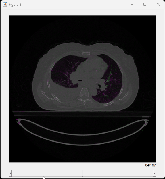
To visually assess the registration, create a falsecolor overlay of the fixed volume and transformed moving volume by using the displayFusedSlices helper function.

displayFusedSlices(medVolReg,medVolExsp)

Scrollable sliceViewer window showing the transverse slices of a fused overlay of the registered volumes.

Display Displacement Field

In addition to the registered image data, the imregdeform function returns an m-by-n-p-by-3 displacement field. The first three dimensions correspond to row, column, and slice indices of the registered volume, and the fourth dimension contains the displacements in the xyz-directions, in pixels. For example, the value dispfield(1,1,1,:) returns a 3-element vector containing the xyz-displacements at the voxel location (1,1,1).

whos dispfield

Convert the displacements from pixel units to millimeters by multiplying each of the x-, y- and z-displacements by the corresponding voxel spacing value.

dispFieldMM = dispField.*reshape(medVolInsp.VoxelSpacing,[1 1 1 3]);

Calculate the magnitude of the displacement by using the vecnorm function. Specify the p input as 2 to calculate the Euclidean distance, and the dimension along which to calculate the norm as 4.

dispMag = vecnorm(dispFieldMM,2,4);

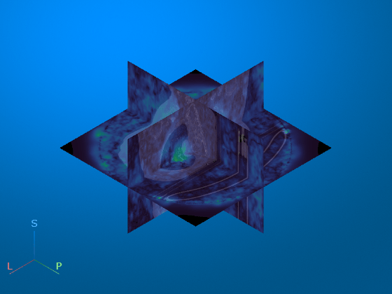
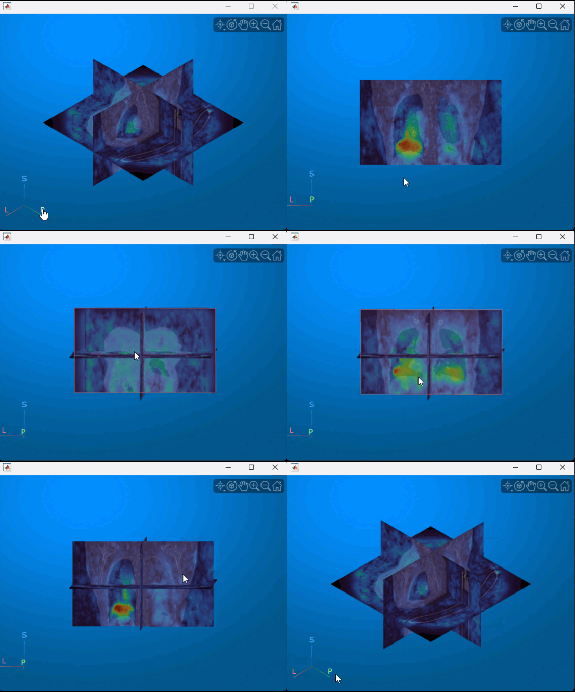
Display the displacement magnitude as an overlay over the original inhale CT volume. The cool heatmap colors indicate smaller displacements, and the warm heatmap regions indicate larger displacements. As expected, the largest respiratory motion occurs within the bottom of the lungs, near the diaphragm. Regions outside the lungs have minimal motion, as the patient did not move or change position within the scanner other than to breathe.

volshow(medVolInsp, ...
    RenderingStyle="SlicePlanes", ...
    OverlayData=dispMag, ...
    OverlayDisplayRangeMode="data-range", ...
    OverlayColormap=turbo(256), ...
    OverlayAlphamap=0.5);

You can interact with the volume display to explore the displacement data, as shown in this animation. To view the coronal plane, click the P axes display indicator. Drag the cursor to rotate the volume slightly out of plane. To scroll through the coronal slices, pause on the coronal slice until it highlights red, then drag it along the anterior/posterior axis. To rotate the volume, click anywhere in the viewer and drag.

Animation showing how to view the coronal plane and scroll through the coronal slices in the interactive viewer window.

Supporting Function

The displayFusedSlices helper function displays a fused overlay of transverse slices of two medicalVolume objects by performing these steps:

To apply uniform scaling to all slices, rescale the voxel intensities to the range [0,1].
Loop through the volumes in the third dimension. At each step, extract the current slice from each volume, and create a fused falsecolor overlay by using imfuse. Specify the Scaling name-value argument as "none" to avoid rescaling the intensity of each slice separately. Add the fused slice to the array fused.
To display the fused image as an RGB volume, reorder the dimensions of the fused image volume so that fusedPermuted is an m-by-n-by-p-by-3 array.
Create a new medicalVolume object that contains the fused image data and the same spatial referencing as the original volumes.
Display the slices of medVolFused in a scrollable figure window.

function displayFusedSlices(medVol1,medVol2)

medVol1Rescale = medVol1;
medVol1Rescale.Voxels = rescale(medVol1.Voxels);

medVol2Rescale = medVol2;
medVol2Rescale.Voxels = rescale(medVol2.Voxels);

for i = 1:size(medVol1Rescale.Voxels,3)
    slice1 = medVol1Rescale.Voxels(:,:,i);
    slice2 = medVol2Rescale.Voxels(:,:,i);
    fused(:,:,:,i) = imfuse(slice1,slice2,method="falsecolor",Scaling="none");
end

fusedPermuted = permute(fused,[1 2 4 3]);
medVolFused = medicalVolume(fusedPermuted,medVol1.VolumeGeometry);
sliceViewer(medVolFused)
end

References

[1] Eslick, Enid M., John Kipritidis, Denis Gradinscak, Mark J. Stevens, Dale L. Bailey, Benjamin Harris, Jeremy T. Booth, and Paul J. Keall. “CT Ventilation as a Functional Imaging Modality for Lung Cancer Radiotherapy (CT-vs-PET-Ventilation-Imaging).” The Cancer Imaging Archive, 2022. https://doi.org/10.7937/3PPX-7S22.

[2] Eslick, Enid M., John Kipritidis, Denis Gradinscak, Mark J. Stevens, Dale L. Bailey, Benjamin Harris, Jeremy T. Booth, and Paul J. Keall. “CT Ventilation Imaging Derived from Breath Hold CT Exhibits Good Regional Accuracy with Galligas PET.” Radiotherapy and Oncology 127, no. 2 (May 2018): 267–73. https://doi.org/10.1016/j.radonc.2017.12.010.

[3] Clark, Kenneth, Bruce Vendt, Kirk Smith, John Freymann, Justin Kirby, Paul Koppel, Stephen Moore, et al. “The Cancer Imaging Archive (TCIA): Maintaining and Operating a Public Information Repository.” Journal of Digital Imaging 26, no. 6 (December 2013): 1045–57. https://doi.org/10.1007/s10278-013-9622-7.