Simulation and Code Generation Using Simulink Coder

Define Plant Model and MPC Controller

Define a SISO plant.

plant = ss(tf([3 1],[1 0.6 1]));

Define the MPC controller for the plant.

Ts = 0.1;   %Sample time
p = 10;     %Prediction horizon
m = 2;      %Control horizon

% Define weights along with input and output constraints.
Weights = struct(MV=0, MVRate=0.01, OV=1);
MV = struct(Min=-Inf, Max=Inf, RateMin=-100, RateMax=100);
OV = struct(Min=-2, Max=2);

% Define mpc object
mpcobj = mpc(plant,Ts,p,m,Weights,MV,OV);

Simulate and Generate Code in Double-Precision

By default, MPC Controller blocks use double-precision data for simulation and code generation.

Simulate the model in Simulink.

mdl1 = "mpc_rtwdemo";
open_system(mdl1)
sim(mdl1)

-->Converting model to discrete time.
-->Assuming output disturbance added to measured output #1 is integrated white noise.
-->"Model.Noise" is empty. Assuming white noise on each measured output.

The controller effort and the plant output are saved into base workspace as variables u and y, respectively.

Build the model with the slbuild command. Use evalc to capture the text output for possible later inspection.

set_param(mdl1,RTWVerbose="off")
disp("Generating C code... Please wait until done.")
txt_out_double = evalc("slbuild(mdl1);");

Generating C code... Please wait until done.

On a Windows® system, an executable file named mpc_rtwdemo.exe appears in the current folder after the build process finishes.

Run the executable.

status = system("." + filesep + mdl1);

** starting the model **
** created mpc_rtwdemo.mat **

After the executable completes successfully (status=0), a data file named mpc_rtwdemo.mat appears in the current directory. This file contains the results from running the executable file. Load the mat file.

load(mdl1)

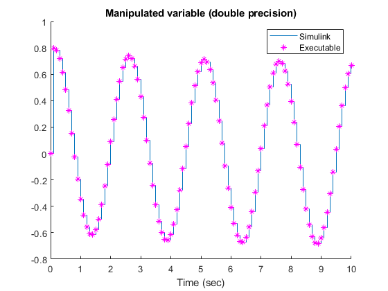
Compare the responses from the executable (rt_u and rt_y) with the responses from the previous simulation in Simulink (u and y).

% Manipulated variable
figure
hold on
stairs(t,u)
stairs(rt_t,rt_u,"*m")
xlabel("Time (sec)")
title("Manipulated variable (double precision)")
legend("Simulink","Executable")
hold off

% Output variable
figure
hold on
stairs(t,y)
stairs(rt_t,rt_y,"*m")
xlabel("Time (sec)")
title("Output variable (double precision)")
legend("Simulink","Executable")
hold off

Display the norm of the differences.

% Manipulated variable
norm(u-rt_u)

% Output Variable
norm(y-rt_y)

ans =

   1.2163e-13


ans =

   2.4816e-14

The responses are numerically equal.

Simulate and Generate Code in Single-Precision

You can also configure the MPC block to use single-precision data in simulation and code generation.

mdl2 = "mpc_rtwdemo_single";
open_system(mdl2)

To do so, set the Output data type property of the MPC Controller block to single.

Simulate the model in Simulink.

sim(mdl2)

The controller effort and the plant output are saved into base workspace as variables u1 and y1, respectively.

Build the model with the slbuild command. Use evalc to capture the text output for possible later inspection.

set_param(mdl2,RTWVerbose="off")
disp("Generating C code... Please wait until done.")
txt_out_single = evalc("slbuild(mdl2);");

Generating C code... Please wait until done.

On a Windows system, an executable file named mpc_rtwdemo_single.exe appears in the temporary directory after the build process finishes.

Run the executable.

status = system("." +  filesep + mdl2);

** starting the model **
** created mpc_rtwdemo_single.mat **

After the executable completes successfully (status=0), a data file named mpc_rtwdemo_single.mat appears in the temporary directory. Load the mat file.

load(mdl2)

Compare the responses from the generated code (rt_u1 and rt_y1) with the responses from the previous simulation in Simulink (u1 and y1).

% Manipulated variable
figure
hold on
stairs(t,u1)
stairs(rt_t,rt_u1,"*m")
xlabel("Time (sec)")
title("Manipulated variable (double precision)")
legend("Simulink","Executable")
hold off

% Output variable
figure
hold on
stairs(t,y1)
stairs(rt_t,rt_y1,"*m")
xlabel("Time (sec)")
title("Output variable (double precision)")
legend("Simulink","Executable")
hold off

Display the norm of the differences.

% Manipulated variable
norm(u1-rt_u1)

% Output Variable
norm(y1-rt_y1)

ans =

  single

  5.2409e-05


ans =

   1.0996e-05

The responses are still practically equal, despite the fact that using a single numeric representation results in the norm of the response difference that is several order of magnitude larger.