Landing a Vehicle Using Multistage Nonlinear MPC
This example shows how to use a multistage nonlinear MPC controller as a planner to find an optimal path that safely lands an airborne vehicle on the ground and then use another multistage nonlinear MPC controller as a feedback controller to follow the generated path and carry out the landing maneuver.
The environment in this example is a 3-DOF lander vehicle represented by a circular disc with mass. The vehicle has two thrusters for forward and rotational motion. Gravity acts vertically downwards, and there are no aerodynamic drag forces. The goal is to first find a path that can safely land the vehicle on the ground at a specified location offline and then execute the landing maneuver at run time.
In this planning and control problem:
Vehicle motion is bounded in X (horizontal axis) from -100 to 100 meters and Y (vertical axis) from 0 to 120 meters.
The goal position is at (0,0) with orientation at 0 radians.
The maximum thrust applied by each thruster can be preconfigured.
The vehicle can have an arbitrary initial position and orientation.
x0 = [-30;60;0;0;0;0];
u0 = [0;0];
Obtain Nonlinear Dynamic Model of the Lander Vehicle
The first-principle nonlinear dynamic model of the vehicle has six states and 2 inputs. Both inputs are manipulated variables.
States:
x: Horizontal position of the center of gravity in metersy: Vertical position of the center of gravity in meterstheta: Tilt angle with respect to the center of gravity in radiansdxdt: Horizontal velocity in meters per seconddydt: Vertical velocity in meters per seconddthetadt: Angular velocity in radians per second
Inputs: # thrust on the left, in Newtons # thrust on the right, in Newtons
The continuous-time model of the lander vehicle is implemented with the LanderVehicleStateFcn function. To speed up optimization, its analytical Jacobian is manually derived in the LanderVehicleStateJacobianFcn file. The model is valid only if the vehicle is above or at the ground ( ).
).
At run time, you assume that all the states are measurable and there is a sensor reading that detects a rough landing (-1), soft landing (1), or airborne (0) condition.
Design Planner and Find Optimal Landing Path
MPC uses an internal model to predict plant behavior in the future. Given the current states of the plant, based on the prediction model, MPC finds an optimal control sequence that minimizes the cost and satisfies all the constraints specified across the prediction horizon. Because MPC finds the state trajectory of the plant in the future, you can use MPC to solve trajectory optimization problems. Such problems include the autonomous parking of a vehicle, motion planning of a robot arm, and finding a landing path for a lander vehicle.
For trajectory optimization problems, the plant, cost function, and constraints are often nonlinear. Therefore, you must formulate and solve the planning problem using nonlinear MPC. You can pass the generated optimal path to a path-following controller as a reference signal, so that it can execute the planned maneuver.
Compared to a generic nonlinear MPC controller, implemented using an nlmpc object, multistage nonlinear MPC provides a more flexible and efficient implementation with staged costs and constraints. This flexibility and efficiency are especially useful for trajectory planning.
A multistage nonlinear MPC controller with prediction horizon p defines p+1 stages, which represent times k (current time) through k+p. For each stage, you can specify stage-specific cost, inequality constraint, and equality constraint functions. Each function depends only on the plant state and input values at the corresponding stage.
Given the current plant states, x[k], the MPC controller finds the manipulated variable (MV) trajectory (from time k to k+p-1) that optimizes the summed stage costs (from time k to k+p) while satisfying all the stage constraints (from time k to k+p).
In this example, select the prediction horizon p and sample time Ts such that the prediction time is p*Ts = 10 seconds.
Ts = 0.2;
pPlanner = 50;
Create a multistage nonlinear MPC controller for the specified prediction horizon and sample time.
planner = nlmpcMultistage(pPlanner,6,2);
planner.Ts = Ts;
Specify prediction model and its analytical Jacobian.
planner.Model.StateFcn = 'LanderVehicleStateFcn';
planner.Model.StateJacFcn = 'LanderVehicleStateJacobianFcn';
Specify hard bounds on the two thrusters. You can adjust the maximum thrust and observe its impact on the landing strategy chosen by the planner. Typical maximum values are between 6 and 10 Newtons. If the maximum thrust is too small, you might not be able to land the vehicle successfully if the initial position is challenging.
planner.MV(1).Min = 0;
planner.MV(1).Max = 8;
planner.MV(2).Min = 0;
planner.MV(2).Max = 8;
To avoid crashing, specify a hard lower bound on the vertical Y position.
planner.States(2).Min = 10;
There are different factors that you can include in your cost function. For example, you can minimize time, fuel consumption, or landing speed. For this example, you define a cost function that optimizes fuel consumption by minimizing the sum of the thrust values. To improve efficiency, you also supply the analytical Jacobian function for the cost.
Use the same cost function for all stages. Because MVs are only valid from stage 1 to stage p, you do not need to define a stage cost for the final stage, p+1.
for ct=1:pPlanner
    planner.Stages(ct).CostFcn = 'LanderVehiclePlannerCostFcn';
    planner.Stages(ct).CostJacFcn = 'LanderVehiclePlannerCostGradientFcn';
end
To ensure a successful landing at the target, specify terminal state for the final stage.
planner.Model.TerminalState = [0;10;0;0;0;0];
In this example, set the maximum number of iterations to a large value to accommodate the large search space and the nonideal default initial guess.
planner.Optimization.SolverOptions.MaxIterations = 1000;
After creating you nonlinear MPC controller, check whether there is any problem with your state, cost, and constraint functions, as well as their analytical Jacobian functions. To do so, call validateFcns functions with random initial plant states and inputs.
validateFcns(planner,rand(6,1),rand(2,1));
Model.StateFcn is OK.
Model.StateJacFcn is OK.
"CostFcn" of the following stages [1 2 3 4 5 6 7 8 9 10 11 12 13 14 15
16 17 18 19 20 21 22 23 24 25 26 27 28 29 30 31 32 33 34 35 36 37 38 39
40 41 42 43 44 45 46 47 48 49 50] are OK.

"CostJacFcn" of the following stages [1 2 3 4 5 6 7 8 9 10 11 12 13 14
15 16 17 18 19 20 21 22 23 24 25 26 27 28 29 30 31 32 33 34 35 36 37 38
39 40 41 42 43 44 45 46 47 48 49 50] are OK.

Analysis of user-provided model, cost, and constraint functions complete.
Compute the optimal landing path using nlmpcmove, which can typically take a few seconds, depending on the initial vehicle position.
fprintf('Lander Vehicle planner running...\n');
tic;
[~,~,info] = nlmpcmove(planner,x0,u0);
t=toc;
fprintf('Calculation Time = %s\n',num2str(t));
fprintf('Objective cost = %s',num2str(info.Cost));
fprintf('ExitFlag = %s',num2str(info.Iterations));
fprintf('Iterations = %s\n',num2str(info.Iterations));
Lander Vehicle planner running...
Calculation Time = 11.7265
Objective cost = 492.9689ExitFlag = 390Iterations = 390
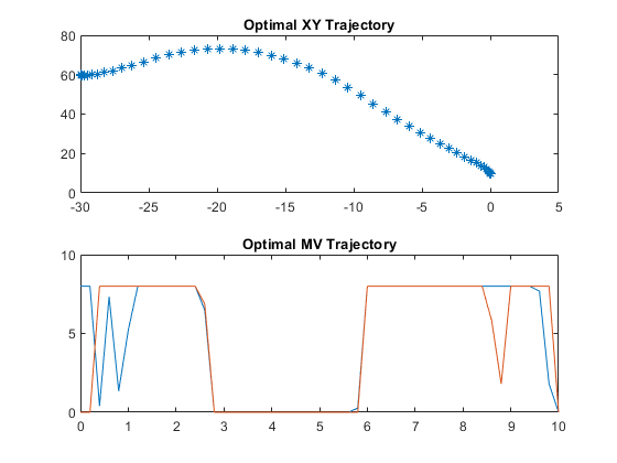
Extract the optimal trajectory from the info structure and plot the result.
figure
subplot(2,1,1)
plot(info.Xopt(:,1),info.Xopt(:,2),'*')
title('Optimal XY Trajectory')
subplot(2,1,2)
plot(info.Topt,info.MVopt(:,1),info.Topt,info.MVopt(:,2))
title('Optimal MV Trajectory')
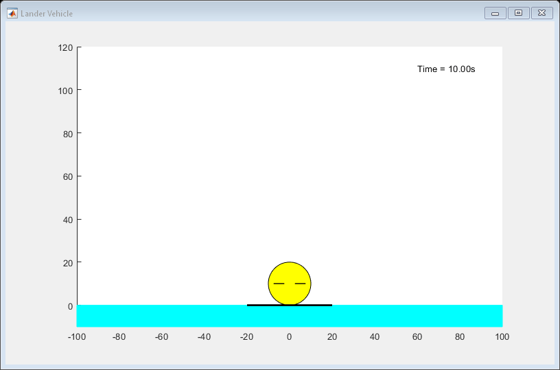
Animate the planned optimal trajectory.
plotobj = LanderVehicleAnimation(6,2);
for ct=1:pPlanner+1
    updatePlot(plotobj,(ct-1)*planner.Ts,info.Xopt(ct,:),info.MVopt(ct,:));
    pause(0.1);
end
Design Lander and Follow the Optimal Path
Like generic nonlinear MPC, you can use multistage nonlinear MPC for reference tracking and disturbance rejection. In this example, you use it to track the optimal trajectory found by the planner. For a path-following problem, the lander does not require a long prediction horizon. Create the controller.
pLander = 10;
lander = nlmpcMultistage(pLander,6,2);
lander.Ts = Ts;
For the path-following controller, the lander has the same prediction model, thrust bounds, and minimum Y position.
lander.Model.StateFcn = 'LanderVehicleStateFcn';
lander.Model.StateJacFcn = 'LanderVehicleStateJacobianFcn';
lander.MV(1).Min = 0;
lander.MV(1).Max = 8;
lander.MV(2).Min = 0;
lander.MV(2).Max = 8;
lander.States(2).Min = 10;
The cost function for the lander is different from that of the planner. The lander uses quadratic cost terms to achieve both tight reference tracking (by penalizing the tracking error) and smooth control actions (by penalizing large changes in the control actions). This lander cost function is implemented in the LanderVehicleCostFcn function. The corresponding manually derived cost gradient function is implemented in LanderVehicleCostGradientFcn.
At run time, you provide the six state trajectory references to the lander as stage parameters. Therefore, specify the number of parameters for each stage.
for ct=1:pLander+1
    lander.Stages(ct).CostFcn = 'LanderVehicleCostFcn';
    lander.Stages(ct).CostJacFcn = 'LanderVehicleCostGradientFcn';
    lander.Stages(ct).ParameterLength = 6;
end
Because changes in control actions are represented by MVRate, you must enable the multistage nonlinear MPC controller to use MVRate values in its in calculations.
lander.UseMVRate = true;
Validate the controller design.
simdata = getSimulationData(lander);
validateFcns(lander,rand(6,1),rand(2,1),simdata);
Model.StateFcn is OK.
Model.StateJacFcn is OK.
"CostFcn" of the following stages [1 2 3 4 5 6 7 8 9 10 11] are OK.

"CostJacFcn" of the following stages [1 2 3 4 5 6 7 8 9 10 11] are OK.

Analysis of user-provided model, cost, and constraint functions complete.
Simulate the landing maneuver in a closed-loop control scenario by iteratively calling nlmpcmove. This simulation assumes that all states are measured. Stop the simulation when the vehicle states are close enough to the target states.
x = x0;
u = u0;
k = 1;
% Extract reference signal as column vector.
references = reshape(info.Xopt',(pPlanner+1)*6,1);
while true

    % Obtain new reference signals.
    simdata.StageParameter = ...
    LanderVehicleReferenceSignal(k,references,pLander);

    % Compute the control action.
    [u,simdata,infoLander] = nlmpcmove(lander,x,u,simdata);

    % Update the animation plot.
    updatePlot(plotobj,(k-1)*Ts,x,u);
    pause(0.1);

    % Simulate the plant to the next state using an ODE solver.
    [~,X] = ode45(@(t,x) LanderVehicleStateFcn(x,u),[0 Ts],x);
    x = X(end,:)';

    % Stop if vehicle has landed.
    if max(abs(x-[0;10;0;0;0;0])) < 1e-2
        % Plot the final vehicle position.
        updatePlot(plotobj,k*Ts,x,zeros(2,1));
        break
    end

    % Move to the next simulation step.
    k = k + 1;
end

Due to the shorter horizon and different cost terms, the landing trajectory slightly differs from the planned trajectory and it takes longer to land. This result is often what happens in such a two-tier control framework with planning and regulation.
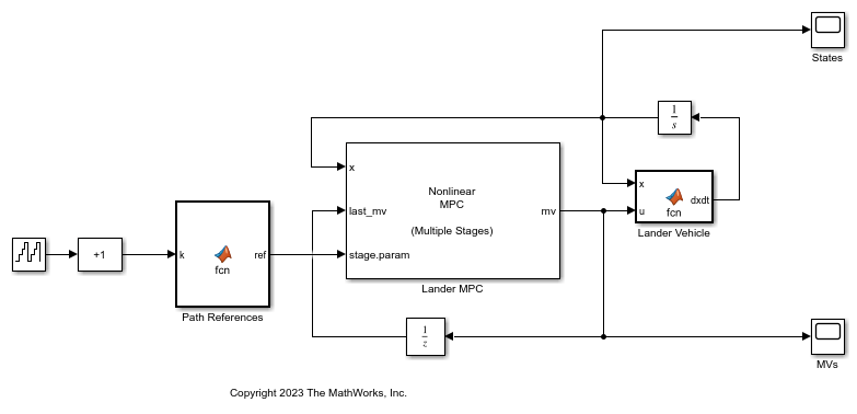
Simulate in Simulink Using Multistage Nonlinear MPC Block
You can implement the same closed-loop simulation in a Simulink® model using the Multistage Nonlinear MPC block.
mdl = 'LanderVehicleSimulation';
open_system(mdl)
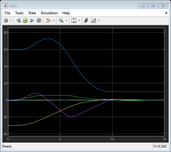
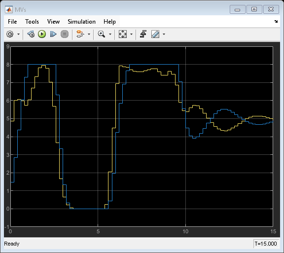
The States scope shows that the plant states are brought to the target states in a reasonable time.
sim(mdl)
open_system([mdl '/States'])
open_system([mdl '/MVs'])
ans =

  Simulink.SimulationOutput:
                   tout: [81x1 double]

     SimulationMetadata: [1x1 Simulink.SimulationMetadata]
           ErrorMessage: [0x0 char]
For real-time applications, you can generate code from the Multistage Nonlinear MPC block.