Specifying Alternative Cost Function with Off-Diagonal Weight Matrices

Define Plant Model and MPC Controller

The linear plant model has two inputs and two outputs.

plant = ss(tf({1,1;1,2},{[1 .5 1],[.7 .5 1];[1 .4 2],[1 2]}));
[A,B,C,D] = ssdata(plant);
Ts = 0.1;               % sampling time
plant = c2d(plant,Ts);  % convert to discrete time

Create an MPC controller with prediction and control horizon of 20 and 2 steps, respectively.

mpcobj = mpc(plant,Ts,20,2);

-->"Weights.ManipulatedVariables" is empty. Assuming default 0.00000.
-->"Weights.ManipulatedVariablesRate" is empty. Assuming default 0.10000.
-->"Weights.OutputVariables" is empty. Assuming default 1.00000.

Define constraints on the manipulated variables and their rates.

mpcobj.MV = struct('Min',{-3;-2},'Max',{3;2},'RateMin',{-100;-100},'RateMax',{100;100});

Specify Non-Diagonal Output Weights

To define non-diagonal output weights, you must select the alternative cost function instead of the standard cost function. The alternative cost function allows off-diagonal weighting, but requires the weights to be identical at each prediction horizon step. For more information on these cost function see Optimization Problem. To select the alternative cost function, you must specify the weight matrices in cell arrays. For more information, see the section on weights in mpc. Specify non-diagonal output weight, corresponding to ((y1-r1)-(y2-r2))^2.

OW = [1 -1]'*[1 -1];
mpcobj.Weights.OutputVariables = {OW};

Specify Non-Diagonal Input Weights

Non-diagonal input weight, corresponding to (u1-u2)^2.

mpcobj.Weights.ManipulatedVariables = {0.5*OW};

Simulate Using SIM Command

Specify simulation time and reference signal.

Tstop = 30;               % simulation time
Tf = round(Tstop/Ts);     % number of simulation steps
r = ones(Tf,1)*[1 2];     % reference trajectory

Run the closed-loop simulation.

[y,t,u] = sim(mpcobj,Tf,r);

-->Assuming output disturbance added to measured output #1 is integrated white noise.
-->Assuming output disturbance added to measured output #2 is integrated white noise.
-->"Model.Noise" is empty. Assuming white noise on each measured output.

Plot the results.

subplot(211)
plot(t,y(:,1)-r(1,1)-y(:,2)+r(1,2));grid
title('(y_1-r_1)-(y_2-r_2)');
subplot(212)
plot(t,u);grid
title('u');

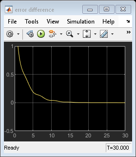
The difference between the two manipulated variable errors tends to zero.

Simulate Using Simulink

Now simulate closed-loop MPC in Simulink®. As expected, results are identical.

mdl = 'mpc_weightsdemo';
open_system(mdl);
sim(mdl)

Close the Simulink model.

bdclose(mdl);