基于问题的大型稀疏二次规划
此示例显示了遇到稀疏问题时使用稀疏算法的价值。矩阵有 n 行,其中您选择 n 作为较大值,以及一些非零对角线带。大小为 n×n 的满矩阵会用尽所有可用内存,但稀疏矩阵则不会出现问题。
问题是最小化 x'*H*x/2 + f'*x,但要满足
x(1) + x(2) + ... + x(n) <= 0,
其中 f = [-1;-2;-3;...;-n]。H 是稀疏对称带状矩阵。
创建稀疏二次矩阵
根据向量 H 的移位创建一个对称循环矩阵 [3,6,2,14,2,6,3],其中 14 位于主对角线上。让矩阵为 n×n,其中 n = 30,000。
n = 3e4;
H2 = speye(n);
H = 3*circshift(H2,-3,2) + 6*circshift(H2,-2,2) + 2*circshift(H2,-1,2)...
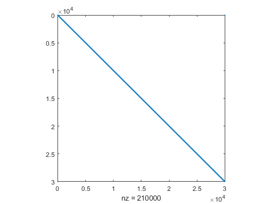
+ 14*H2 + 2*circshift(H2,1,2) + 6*circshift(H2,2,2) + 3*circshift(H2,3,2);查看稀疏矩阵结构。
spy(H)
创建优化变量和问题
创建优化变量 x 和问题 qprob。
x = optimvar('x',n);
qprob = optimproblem;
创建目标函数和约束。将目标和约束放入 qprob。
f = 1:n;
obj = 1/2*x'*H*x - f*x;
qprob.Objective = obj;
cons = sum(x) <= 0;
qprob.Constraints = cons;
求解问题
使用默认的 interior-point-convex' 算法和稀疏线性代数求解二次规划问题。为了防止求解器过早停止,请将 StepTolerance 选项设置为 0。
options = optimoptions('quadprog','Algorithm','interior-point-convex',...
    'LinearSolver','sparse','StepTolerance',0);
[sol,fval,exitflag,output,lambda] = solve(qprob,'Options',options);
Minimum found that satisfies the constraints.

Optimization completed because the objective function is non-decreasing in
feasible directions, to within the value of the optimality tolerance,
and constraints are satisfied to within the value of the constraint tolerance.

<stopping criteria details>
检查解
查看与线性不等式约束相关的目标函数值、迭代次数和拉格朗日乘数。
fprintf('The objective function value is %d.\nThe number of iterations is %d.\nThe Lagrange multiplier is %d.\n',...
    fval,output.iterations,lambda.Constraints)
The objective function value is -3.133073e+10.
The number of iterations is 7.
The Lagrange multiplier is 1.500050e+04.
评估约束以查看解是否在边界上。
fprintf('The linear inequality constraint sum(x) has value %d.\n',sum(sol.x))The linear inequality constraint sum(x) has value 7.599738e-09.
解分量的总和为零,在公差范围内。
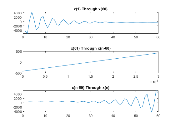
解 x 有三个区域:初始部分、最终部分和覆盖大部分解的近似线性部分。绘制三个区域。
subplot(3,1,1)
plot(sol.x(1:60))
title('x(1) Through x(60)')
subplot(3,1,2)
plot(sol.x(61:n-60))
title('x(61) Through x(n-60)')
subplot(3,1,3)
plot(sol.x(n-59:n))
title('x(n-59) Through x(n)')