使用 Parallel Computing Toolbox 最小化高成本优化问题
R2026a此示例说明如何使用 Optimization Toolbox™ 和 Global Optimization Toolbox 中的函数来加速高成本优化问题的最小化。在示例的第一部分,通过以串行方式计算函数来求解优化问题,在示例的第二部分,通过并行计算函数以使用并行 for 循环 (parfor) 功能来求解相同的问题。可以比较在两种情况下优化函数所花费的时间。
高成本优化问题
出于本示例的目的,将用四个变量来求解问题,在这个过程中,通过暂停人为地增加目标函数和约束函数的成本。
function f = expensive_objfun(x)
% Simulate an expensive function by pausing.
pause(0.1)
% Evaluate objective function.
f = exp(x(1)) * (4*x(3)^2 + 2*x(4)^2 + 4*x(1)*x(2) + 2*x(2) + 1);
end

function [ineqnonlin,eqnonlin] = expensive_confun(x)
% Simulate an expensive function by pausing.
pause(0.1);
% Evaluate constraints.
ineqnonlin = [1.5 + x(1)*x(2)*x(3) - x(1) - x(2) - x(4);
     -x(1)*x(2) + x(4) - 10];
% No nonlinear equality constraints:
eqnonlin = [];
end
使用 fmincon 进行最小化
测量 fmincon 以串行方式运行所用的时间,以便可以将其与并行时间进行比较。
startPoint = [-1 1 1 -1];
options = optimoptions("fmincon",Display="iter");
startTime = tic;
xsol = fmincon(@expensive_objfun,startPoint,[],[],[],[],[],[],@expensive_confun,options);
                                            First-order      Norm of
 Iter F-count            f(x)  Feasibility   optimality         step
    0       5    1.839397e+00    1.500e+00    3.211e+00
    1      11   -9.760099e-01    3.708e+00    7.902e-01    2.362e+00
    2      16   -1.480976e+00    0.000e+00    8.344e-01    1.069e+00
    3      21   -2.601599e+00    0.000e+00    8.390e-01    1.218e+00
    4      29   -2.823630e+00    0.000e+00    2.598e+00    1.118e+00
    5      34   -3.905338e+00    0.000e+00    1.210e+00    7.302e-01
    6      39   -6.212992e+00    3.934e-01    7.372e-01    2.405e+00
    7      44   -5.948761e+00    0.000e+00    1.784e+00    1.905e+00
    8      49   -6.940062e+00    1.233e-02    7.668e-01    7.553e-01
    9      54   -6.973887e+00    0.000e+00    2.549e-01    3.920e-01
   10      59   -7.142993e+00    0.000e+00    1.903e-01    4.735e-01
   11      64   -7.155325e+00    0.000e+00    1.365e-01    2.626e-01
   12      69   -7.179122e+00    0.000e+00    6.336e-02    9.115e-02
   13      74   -7.180116e+00    0.000e+00    1.069e-03    4.670e-02
   14      79   -7.180409e+00    0.000e+00    7.799e-04    2.815e-03
   15      84   -7.180410e+00    0.000e+00    6.607e-06    3.121e-04

Local minimum found that satisfies the constraints.

Optimization completed because the objective function is non-decreasing in
feasible directions, to within the value of the optimality tolerance,
and constraints are satisfied to within the value of the constraint tolerance.

<stopping criteria details>
time_fmincon_sequential = toc(startTime);
fprintf("Serial fmincon optimization takes %g seconds.\n",time_fmincon_sequential);
Serial fmincon optimization takes 18.9224 seconds.
使用遗传算法进行最小化
由于 ga 通常比 fmincon 需要更多函数计算,因此将从此问题中删除高成本约束,改为执行无约束优化。为约束传递空矩阵 []。此外,将 ga 的最大代数限制为 15,以便 ga 可以在合理的时间内终止。测量 ga 运行所用的时间,以便您可以将其与并行 ga 计算进行比较。请注意,运行 ga 需要 Global Optimization Toolbox。
rng default % for reproducibility
try
    gaAvailable = false;
    nvar = 4;
    gaoptions = optimoptions("ga",MaxGenerations=15,Display="iter");
    startTime = tic;
gasol = ga(@expensive_objfun,nvar,[],[],[],[],[],[],[],gaoptions);
    time_ga_sequential = toc(startTime);
fprintf("Serial ga optimization takes %g seconds.\n",time_ga_sequential);
    gaAvailable = true;
catch ME
    warning(message("optim:optimdemos:optimparfor:gaNotFound"));
end
Single objective optimization:
4 Variables

Options:
CreationFcn:       @gacreationuniform
CrossoverFcn:      @crossoverscattered
SelectionFcn:      @selectionstochunif
MutationFcn:       @mutationgaussian

                                  Best           Mean      Stall
Generation      Func-count        f(x)           f(x)    Generations
    1              100      -5.546e+05       1.483e+15        0
    2              147      -5.581e+17      -1.116e+16        0
    3              194      -7.556e+17       6.679e+22        0
    4              241      -7.556e+17      -7.195e+16        1
    5              288      -9.381e+27      -1.876e+26        0
    6              335      -9.673e+27      -7.497e+26        0
    7              382      -4.511e+36      -9.403e+34        0
    8              429      -5.111e+36      -3.011e+35        0
    9              476      -7.671e+36       9.346e+37        0
   10              523       -1.52e+43      -3.113e+41        0
   11              570      -2.273e+45       -4.67e+43        0
   12              617      -2.589e+47      -6.281e+45        0
   13              664      -2.589e+47      -1.015e+46        1
   14              711      -8.149e+47      -5.855e+46        0
   15              758      -9.503e+47       -1.29e+47        0
ga stopped because it exceeded options.MaxGenerations.
Serial ga optimization takes 83.4899 seconds.
设置 Parallel Computing Toolbox
如果 Parallel Computing Toolbox™ 可用并且有并行工作单元池,则 Optimization Toolbox 中用于逼近导数的函数的有限差分是使用 parfor 功能以并行方式完成的。同样,Global Optimization Toolbox 中的 ga、gamultiobj 和 patternsearch 求解器以并行方式计算函数。要使用 parfor 函数,请使用 parpool 函数来设置并行环境。发布此示例的计算机有四个核,因此 parpool 会启动四个 MATLAB® 工作单元。如果在运行此示例时已有并行池,就使用该池;有关详细信息,请参阅 parpool 的文档。
if max(size(gcp)) == 0 % parallel pool needed
    parpool % create the parallel pool
end
使用并行 fmincon 进行最小化
为了使用并行 fmincon 函数最小化高成本优化问题,您需要显式指示我们的目标函数和约束函数可以以并行方式进行计算,并且您希望 fmincon 尽可能使用其并行功能。目前,有限差分可以以并行方式完成。测量并行 fmincon 运行所用的时间,以便您可以将其与串行 fmincon 运行进行比较。
options = optimoptions(options,UseParallel=true);
startTime = tic;
xsol = fmincon(@expensive_objfun,startPoint,[],[],[],[],[],[],@expensive_confun,options);
                                            First-order      Norm of
 Iter F-count            f(x)  Feasibility   optimality         step
    0       5    1.839397e+00    1.500e+00    3.211e+00
    1      11   -9.760099e-01    3.708e+00    7.902e-01    2.362e+00
    2      16   -1.480976e+00    0.000e+00    8.344e-01    1.069e+00
    3      21   -2.601599e+00    0.000e+00    8.390e-01    1.218e+00
    4      29   -2.823630e+00    0.000e+00    2.598e+00    1.118e+00
    5      34   -3.905338e+00    0.000e+00    1.210e+00    7.302e-01
    6      39   -6.212992e+00    3.934e-01    7.372e-01    2.405e+00
    7      44   -5.948761e+00    0.000e+00    1.784e+00    1.905e+00
    8      49   -6.940062e+00    1.233e-02    7.668e-01    7.553e-01
    9      54   -6.973887e+00    0.000e+00    2.549e-01    3.920e-01
   10      59   -7.142993e+00    0.000e+00    1.903e-01    4.735e-01
   11      64   -7.155325e+00    0.000e+00    1.365e-01    2.626e-01
   12      69   -7.179122e+00    0.000e+00    6.336e-02    9.115e-02
   13      74   -7.180116e+00    0.000e+00    1.069e-03    4.670e-02
   14      79   -7.180409e+00    0.000e+00    7.799e-04    2.815e-03
   15      84   -7.180410e+00    0.000e+00    6.607e-06    3.121e-04

Local minimum found that satisfies the constraints.

Optimization completed because the objective function is non-decreasing in
feasible directions, to within the value of the optimality tolerance,
and constraints are satisfied to within the value of the constraint tolerance.

<stopping criteria details>
time_fmincon_parallel = toc(startTime);
fprintf("Parallel fmincon optimization takes %g seconds.\n",time_fmincon_parallel);
Parallel fmincon optimization takes 10.7073 seconds.
使用并行遗传算法进行最小化
为了使用 ga 函数最小化高成本优化问题,您需要显式指示目标函数可以并行计算,并且您希望 ga 尽可能使用其并行功能。要使用并行 ga,您必须确保 Vectorized 选项设置为默认值 ("off")。测量 ga 运行所用的时间,以便您可以将其与串行 ga 运行进行比较。尽管由于 ga 使用随机数生成器,这次运行可能与串行运行不同,但两次运行中高成本的函数计算次数是相同的。请注意,运行 ga 需要 Global Optimization Toolbox。
rng default % To get the same evaluations as the previous run
if gaAvailable
    gaoptions = optimoptions(gaoptions,UseParallel=true);
    startTime = tic;
gasol = ga(@expensive_objfun,nvar,[],[],[],[],[],[],[],gaoptions);
    time_ga_parallel = toc(startTime);
fprintf("Parallel ga optimization takes %g seconds.\n",time_ga_parallel);
end
Single objective optimization:
4 Variables

Options:
CreationFcn:       @gacreationuniform
CrossoverFcn:      @crossoverscattered
SelectionFcn:      @selectionstochunif
MutationFcn:       @mutationgaussian

                                  Best           Mean      Stall
Generation      Func-count        f(x)           f(x)    Generations
    1              100      -5.546e+05       1.483e+15        0
    2              147      -5.581e+17      -1.116e+16        0
    3              194      -7.556e+17       6.679e+22        0
    4              241      -7.556e+17      -7.195e+16        1
    5              288      -9.381e+27      -1.876e+26        0
    6              335      -9.673e+27      -7.497e+26        0
    7              382      -4.511e+36      -9.403e+34        0
    8              429      -5.111e+36      -3.011e+35        0
    9              476      -7.671e+36       9.346e+37        0
   10              523       -1.52e+43      -3.113e+41        0
   11              570      -2.273e+45       -4.67e+43        0
   12              617      -2.589e+47      -6.281e+45        0
   13              664      -2.589e+47      -1.015e+46        1
   14              711      -8.149e+47      -5.855e+46        0
   15              758      -9.503e+47       -1.29e+47        0
ga stopped because it exceeded options.MaxGenerations.
Parallel ga optimization takes 22.4566 seconds.
比较串行和并行时间
X = [time_fmincon_sequential time_fmincon_parallel];
Y = [time_ga_sequential time_ga_parallel];
t = [0 1];
plot(t,X,"r--",t,Y,"k-")
ylabel("Time in seconds")
legend("fmincon","ga")
ax = gca;
ax.XTick = [0 1];
ax.XTickLabel = ["Serial" "Parallel"];
axis([0 1 0 ceil(max([X Y]))])
title("Serial Vs. Parallel Times")
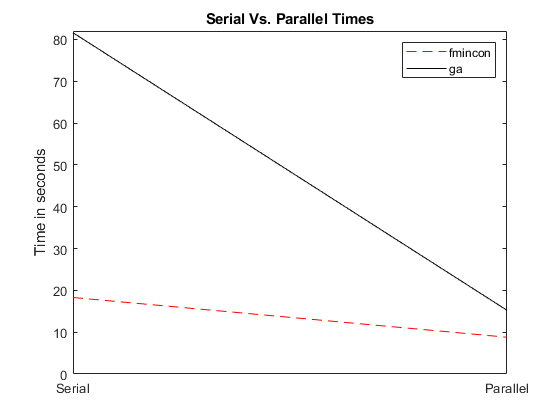
通过 parfor 利用并行函数计算提高了 fmincon 和 ga 的效率。对于高成本的目标函数和约束函数,这种改进通常更明显。

