具有边界约束的二次规划问题:基于问题
此示例说明如何表示和求解具有二次目标函数的可伸缩边界约束问题。该示例还说明使用几种算法的求解行为。问题可以有任意个数的变量;变量个数决定了问题的规模。对于此示例的基于求解器的版本,请参阅有约束约束的二次最小化。
作为问题变量个数 n 的函数,目标函数为
创建问题
创建一个名为 x 的问题变量,它包含 400 个分量。此外,为目标函数创建一个名为 objec 的表达式。除了允许 无界之外,将每个变量的下界设置为 0,上界设置为 0.9。
n = 400;
x = optimvar("x",n,LowerBound=0,UpperBound=0.9);
x(n).LowerBound = -Inf;
x(n).UpperBound = Inf;
prevtime = 1:n-1;
nexttime = 2:n;
objec = 2*sum(x.^2) - 2*sum(x(nexttime).*x(prevtime)) - 2*x(1) - 2*x(end);
创建一个名为 qprob 的优化问题。在问题中包含目标函数。
qprob = optimproblem(Objective=objec);
创建选项对象,其中指定 quadprog "trust-region-reflective" 算法且不显示输出。创建一个大约位于边界中心的初始点。
opts = optimoptions("quadprog",Algorithm="trust-region-reflective",Display="off");
x0 = 0.5*ones(n,1);
x00 = struct("x",x0);
求解问题并检查解
求解。
[sol,qfval,qexitflag,qoutput] = solve(qprob,x00,Options=opts);
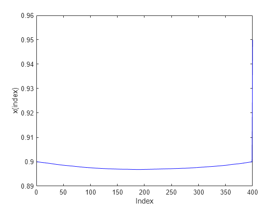
绘制解。
plot(sol.x,"b-")
xlabel("Index")
ylabel("x(index)")
报告退出标志、迭代次数和共轭梯度迭代次数。
fprintf("Exit flag = %d, iterations = %d, cg iterations = %d\n",...
    double(qexitflag),qoutput.iterations,qoutput.cgiterations)
Exit flag = 3, iterations = 20, cg iterations = 1813
可以看到有大量的共轭梯度迭代。
调整选项以提高效率
通过将 SubproblemAlgorithm 选项设置为 "factorization",减少共轭梯度迭代的次数。此选项使得求解器使用成本更高的内部求解方法,该方法避免了使用共轭梯度步,因此在总体上节省了时间。
opts.SubproblemAlgorithm = "factorization";
[sol2,qfval2,qexitflag2,qoutput2] = solve(qprob,x00,Options=opts);
fprintf("Exit flag = %d, iterations = %d, cg iterations = %d\n",...
    double(qexitflag2),qoutput2.iterations,qoutput2.cgiterations)
Exit flag = 3, iterations = 10, cg iterations = 0
迭代次数和共轭梯度迭代次数都减少了。
将解与 "interior-point" 解进行比较
将这些解与使用默认 "interior-point" 算法获得的解进行比较。"interior-point" 算法不使用初始点,因此不会将 x00 传递给 solve。
opts = optimoptions("quadprog",Algorithm="interior-point-convex",Display="off");
[sol3,qfval3,qexitflag3,qoutput3] = solve(qprob,Options=opts);
fprintf("Exit flag = %d, iterations = %d, cg iterations = %d\n",...
    double(qexitflag3),qoutput3.iterations,0)
Exit flag = 1, iterations = 8, cg iterations = 0
middle = floor(n/2);
fprintf("The three solutions are slightly different.\nThe middle component is %f, %f, or %f.\n",...
    sol.x(middle),sol2.x(middle),sol3.x(middle))
The three solutions are slightly different.
The middle component is 0.897338, 0.898801, or 0.857389.
fprintf("The relative norm of sol - sol2 is %f.\n",norm(sol.x-sol2.x)/norm(sol.x))The relative norm of sol - sol2 is 0.001116.
fprintf("The relative norm of sol2 - sol3 is %f.\n",norm(sol2.x-sol3.x)/norm(sol2.x))The relative norm of sol2 - sol3 is 0.036007.
fprintf("The three objective function values are %f, %f, and %f.\n" ...
    +"The ''interior-point'' algorithm is slightly less accurate.",qfval,qfval2,qfval3)
The three objective function values are -1.985000, -1.985000, and -1.984963.
The ''interior-point'' algorithm is slightly less accurate.