基于求解器的投资组合优化问题的二次规划

此示例说明如何使用 quadprog 中的内点二次规划算法来求解投资组合优化问题。函数 quadprog 属于 Optimization Toolbox™。

在此示例中定义问题的矩阵是稠密矩阵；然而，quadprog 中的内点算法也可以利用问题矩阵的稀疏性来提高速度。有关稀疏示例，请参阅Large Sparse Quadratic Program with Interior Point Algorithm。

二次模型

假设有种不同资产。资产回报率是随机变量，预期值为。问题是在指定的最低预期回报率约束下，找出在每项资产上的投资比例为多少，才能将风险降至最低。

让表示资产回报率的协方差矩阵。

经典的均值-方差模型是在一组约束条件下最小化投资组合风险，风险可由下式衡量

$\frac{1}{2}x^T C x$

其中约束如下：

预期回报率不应低于投资者期望的最低投资组合回报率，

$\sum_{i=1}^n m_i \; x_i \ge r,$

投资组合比例的总和应为 1，

$\sum_{i=1}^n x_i = 1,$

而且作为比例（或百分比），它们应为介于 0 和 1 之间的数字，

$0 \le x_i \le 1, \;\;\; i = 1 \ldots n.$

由于最小化投资组合风险的目标函数是二次型的，而约束是线性的，因此该优化问题是二次规划，即 QP。

225 项资产问题

现在让我们求解包含 225 项资产的 QP。该数据集来自 OR-Library [Chang, T.-J., Meade, N., Beasley, J.E. and Sharaiha, Y.M., "Heuristics for cardinality constrained portfolio optimisation" Computers & Operations Research 27 (2000) 1271-1302]。

我们加载数据集，然后按 quadprog 所需的格式设置约束。在此数据集中，回报率的范围在 -0.008489 和 0.003971 之间；我们在两者之间选择一个期望的回报率，例如 0.002 (0.2%)。

加载存储在 MAT 文件中的数据集。

load('port5.mat','Correlation','stdDev_return','mean_return')

基于相关矩阵计算协方差矩阵。

Covariance = Correlation .* (stdDev_return * stdDev_return');
nAssets = numel(mean_return); r = 0.002;     % number of assets and desired return
Aeq = ones(1,nAssets); beq = 1;              % equality Aeq*x = beq
Aineq = -mean_return'; bineq = -r;           % inequality Aineq*x <= bineq
lb = zeros(nAssets,1); ub = ones(nAssets,1); % bounds lb <= x <= ub
c = zeros(nAssets,1);                        % objective has no linear term; set it to zero

在 Quadprog 中选择内点算法

为了使用内点算法求解 QP，我们将选项算法设置为 'interior-point-convex'。

options = optimoptions('quadprog','Algorithm','interior-point-convex');

求解 225 项资产问题

我们现在设置一些额外的选项，并调用求解器 quadprog。

设置附加选项：打开迭代输出，并设置更严格的最优性终止容差。

options = optimoptions(options,'Display','iter','TolFun',1e-10);

调用求解器并测量挂钟时间。

tic
[x1,fval1] = quadprog(Covariance,c,Aineq,bineq,Aeq,beq,lb,ub,[],options);
toc

 Iter            Fval  Primal Infeas    Dual Infeas  Complementarity  
    0    2.384401e+01   2.253410e+02   1.337381e+00     1.000000e+00  
    1    1.338822e-03   7.394864e-01   4.388791e-03     1.038098e-02  
    2    1.186079e-03   6.443975e-01   3.824446e-03     8.727381e-03  
    3    5.923977e-04   2.730703e-01   1.620650e-03     1.174211e-02  
    4    5.354880e-04   5.303581e-02   3.147632e-04     1.549549e-02  
    5    5.181994e-04   2.651791e-05   1.573816e-07     2.848171e-04  
    6    5.066191e-04   9.285375e-06   5.510794e-08     1.041224e-04  
    7    3.923090e-04   7.619855e-06   4.522322e-08     5.536006e-04  
    8    3.791545e-04   1.770065e-06   1.050519e-08     1.382075e-04  
    9    2.923749e-04   8.850312e-10   5.252599e-12     3.858983e-05  
   10    2.277722e-04   4.431702e-13   2.627914e-15     6.204101e-06  
   11    1.992243e-04   2.229120e-16   2.127959e-18     4.391483e-07  
   12    1.950468e-04   3.339343e-16   1.456847e-18     1.429441e-08  
   13    1.949141e-04   3.330669e-16   1.239159e-18     9.731942e-10  
   14    1.949121e-04   8.886121e-16   6.938894e-18     2.209702e-12  

Minimum found that satisfies the constraints.

Optimization completed because the objective function is non-decreasing in 
feasible directions, to within the value of the optimality tolerance,
and constraints are satisfied to within the value of the constraint tolerance.

Elapsed time is 0.165264 seconds.

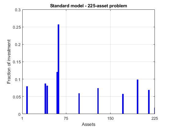
绘制结果。

plotPortfDemoStandardModel(x1)

具有组约束的 225 项资产问题

我们现在向模型增加组约束，即要求投资者 30% 的资金必须投资于资产 1 至 75，30% 投资于资产 76 至 150，30% 投资于资产 151 至 225。每组资产可以是不同行业，例如技术、汽车和制药。实现此新要求的约束是

$\sum_{i=1}^{75} x_i \ge 0.3, \qquad$ $\sum_{i=76}^{150} x_i \ge 0.3, \qquad$ $\sum_{i=151}^{225} x_i \ge 0.3.$

向现有等式添加组约束。

Groups = blkdiag(ones(1,nAssets/3),ones(1,nAssets/3),ones(1,nAssets/3));
Aineq = [Aineq; -Groups];         % convert to <= constraint
bineq = [bineq; -0.3*ones(3,1)];  % by changing signs

调用求解器并测量挂钟时间。

tic
[x2,fval2] = quadprog(Covariance,c,Aineq,bineq,Aeq,beq,lb,ub,[],options);
toc

 Iter            Fval  Primal Infeas    Dual Infeas  Complementarity  
    0    2.384401e+01   4.464410e+02   1.337324e+00     1.000000e+00  
    1    1.346872e-03   1.474737e+00   4.417606e-03     3.414918e-02  
    2    1.190113e-03   1.280566e+00   3.835962e-03     2.934585e-02  
    3    5.990845e-04   5.560762e-01   1.665738e-03     1.320038e-02  
    4    3.890097e-04   2.780381e-04   8.328691e-07     7.287370e-03  
    5    3.887354e-04   1.480950e-06   4.436215e-09     4.641988e-05  
    6    3.387787e-04   8.425389e-07   2.523843e-09     2.578178e-05  
    7    3.089240e-04   2.707587e-07   8.110632e-10     9.217509e-06  
    8    2.639458e-04   6.586817e-08   1.973095e-10     6.509001e-06  
    9    2.252657e-04   2.225507e-08   6.666551e-11     6.783212e-06  
   10    2.105838e-04   5.811527e-09   1.740855e-11     1.967570e-06  
   11    2.024362e-04   4.129834e-12   1.237133e-14     5.924109e-08  
   12    2.009703e-04   4.289104e-15   1.409629e-17     6.353270e-10  
   13    2.009650e-04   3.903128e-16   6.938894e-18     1.596041e-13  

Minimum found that satisfies the constraints.

Optimization completed because the objective function is non-decreasing in 
feasible directions, to within the value of the optimality tolerance,
and constraints are satisfied to within the value of the constraint tolerance.

Elapsed time is 0.058514 seconds.

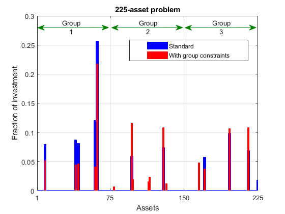
绘制结果，叠加在先前问题的结果上。

plotPortfDemoGroupModel(x1,x2);

迄今为止结果摘要

我们从第二个条形图中看到，由于存在额外的组约束，与第一个投资组合相比，现在投资组合在三个资产组中的分布更均匀。这种强加的多样化也导致风险略微增加，这是通过目标函数来测量的（请参阅两次运行的迭代输出中最后一次迭代的标记为“f(x)”的列）。

使用随机数据的 1000 项资产问题

为了说明 quadprog 的内点算法如何处理更大型的问题，我们将使用包含 1000 项资产的随机生成的数据集。我们使用 MATLAB® 中的 gallery 函数生成随机相关矩阵（对称、半正定矩阵，对角线元素为 1）。

重置随机流以实现可再现性。

rng(0,'twister');
nAssets = 1000; % desired number of assets

生成 -0.1 到 0.4 之间的回报率均值数据。

a = -0.1; b = 0.4;
mean_return = a + (b-a).*rand(nAssets,1);

生成 0.08 到 0.6 之间的回报率标准差数据。

a = 0.08; b = 0.6;
stdDev_return = a + (b-a).*rand(nAssets,1);
% Correlation matrix, generated using Correlation = gallery('randcorr',nAssets).
% (Generating a correlation matrix of this size takes a while, so we load
% a pre-generated one instead.)
load('correlationMatrixDemo.mat','Correlation');
% Calculate covariance matrix from correlation matrix.
Covariance = Correlation .* (stdDev_return * stdDev_return');

定义并求解随机生成的 1000 项资产问题

我们现在定义标准的 QP 问题（此处没有组约束）并求解。

r = 0.15;                                     % desired return
Aeq = ones(1,nAssets); beq = 1;               % equality Aeq*x = beq
Aineq = -mean_return'; bineq = -r;            % inequality Aineq*x <= bineq
lb = zeros(nAssets,1); ub = ones(nAssets,1);  % bounds lb <= x <= ub
c = zeros(nAssets,1);                         % objective has no linear term; set it to zero

调用求解器并测量挂钟时间。

tic
x3 = quadprog(Covariance,c,Aineq,bineq,Aeq,beq,lb,ub,[],options);
toc

 Iter            Fval  Primal Infeas    Dual Infeas  Complementarity  
    0    7.083800e+01   1.142266e+03   1.610094e+00     1.000000e+00  
    1    5.603619e-03   7.133717e+00   1.005541e-02     9.857295e-02  
    2    1.076070e-04   3.566858e-03   5.027704e-06     9.761758e-03  
    3    1.068230e-04   2.513041e-06   3.542285e-09     8.148386e-06  
    4    7.257177e-05   1.230928e-06   1.735068e-09     3.979480e-06  
    5    3.610589e-05   2.634706e-07   3.713779e-10     1.175001e-06  
    6    2.077811e-05   2.562892e-08   3.612553e-11     5.617206e-07  
    7    1.611590e-05   4.711751e-10   6.641535e-13     5.652911e-08  
    8    1.491953e-05   4.926282e-12   6.940520e-15     2.427880e-09  
    9    1.477930e-05   1.317835e-13   1.852562e-16     2.454705e-10  
   10    1.476910e-05   8.049117e-16   9.619336e-19     2.786060e-11  

Minimum found that satisfies the constraints.

Optimization completed because the objective function is non-decreasing in 
feasible directions, to within the value of the optimality tolerance,
and constraints are satisfied to within the value of the constraint tolerance.

Elapsed time is 0.840664 seconds.