2-D Solution and Gradient Plots with MATLAB Functions

Open Live Script

You can interpolate the solution and, if needed, its gradient in separate steps, and then plot the results by using MATLAB® functions, such as surf, mesh, quiver, and so on. For example, solve the same scalar elliptic problem $- Δ u = 1$ on the L-shaped membrane with zero Dirichlet boundary conditions. Interpolate the solution and its gradient, and then plot the results.

Create the PDE model, 2-D geometry, and mesh. Specify boundary conditions and coefficients. Solve the PDE problem.

model = createpde;
geometryFromEdges(model,@lshapeg);
applyBoundaryCondition(model,"dirichlet", ...
                       Edge=1:model.Geometry.NumEdges, ...
                       u=0);
c = 1;
a = 0;
f = 1;
specifyCoefficients(model,m=0,d=0,c=c,a=a,f=f);
generateMesh(model,Hmax=0.05);
results = solvepde(model);

Interpolate the solution and its gradients to a dense grid from -1 to 1 in each direction.

v = linspace(-1,1,101);
[X,Y] = meshgrid(v);
querypoints = [X(:),Y(:)]';
uintrp = interpolateSolution(results,querypoints);

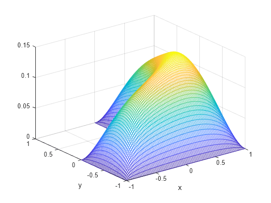
Plot the resulting solution on a mesh.

uintrp = reshape(uintrp,size(X));
mesh(X,Y,uintrp)
xlabel("x")
ylabel("y")

Figure contains an axes object. The axes object with xlabel x, ylabel y contains an object of type surface.

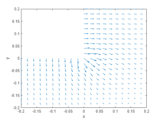
Interpolate gradients of the solution to the grid from -1 to 1 in each direction. Plot the result using quiver.

[gradx,grady] = evaluateGradient(results,querypoints);
figure
quiver(X(:),Y(:),gradx,grady)
xlabel("x")
ylabel("y")

Zoom in to see more details. For example, restrict the range to [-0.2,0.2] in each direction.

axis([-0.2 0.2 -0.2 0.2])

Figure contains an axes object. The axes object with xlabel x, ylabel y contains an object of type quiver.

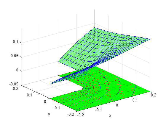
Plot the solution and the gradients on the same range.

figure
h1 = meshc(X,Y,uintrp);
set(h1,FaceColor="g",EdgeColor="b")
xlabel("x")
ylabel("y")
alpha(0.5)
hold on

Z = -0.05*ones(size(X));
gradz = zeros(size(gradx));

h2 = quiver3(X(:),Y(:),Z(:),gradx,grady,gradz);
set(h2,Color="r")
axis([-0.2,0.2,-0.2,0.2])

Figure contains an axes object. The axes object with xlabel x, ylabel y contains 3 objects of type surface, contour, quiver.

Slice of the solution plot along the line x = y.

figure
mesh(X,Y,uintrp)
xlabel("x")
ylabel("y")
alpha(0.25)
hold on

z = linspace(0,0.15,101);
Z = meshgrid(z);
surf(X,X,Z')

view([-20 -45 15])
colormap winter

Figure contains an axes object. The axes object with xlabel x, ylabel y contains 2 objects of type surface.

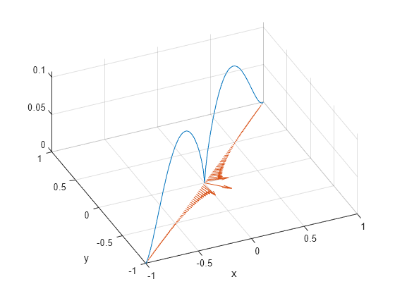
Plot the interpolated solution along the line.

figure
xq = v;
yq = v;
uintrp = interpolateSolution(results,xq,yq);

plot3(xq,yq,uintrp)
grid on
xlabel("x")
ylabel("y")

Interpolate gradients of the solution along the same line and add them to the solution plot.

[gradx,grady] = evaluateGradient(results,xq,yq);

gradx = reshape(gradx,size(xq));
grady = reshape(grady,size(yq));

hold on
quiver(xq,yq,gradx,grady)
view([-20 -45 75])

Figure contains an axes object. The axes object with xlabel x, ylabel y contains 2 objects of type line, quiver.