3-D Multidomain Geometry from 2-D Geometry

This example shows how to create a 3-D multidomain geometry by extruding a 2-D geometry imported from STL data. The original 2-D geometry represents a cooled turbine blade section defined by a 2-D profile.

Before extruding the geometry, this example modifies the original 2-D profile as follows:

Import the geometry.

g = fegeometry("CooledBlade2D.STL");

Plot the geometry with the face labels.

figure
pdegplot(g,FaceLabels="on")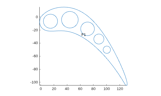

Translate the geometry to align the tip of the blade with the origin.

tip = [1.802091,-127.98192215];
g = translate(g,tip);

Rotate the geometry to align the chord with the x-axis.

angle = -36.26005;
g = rotate(g,angle);

Scale the geometry to convert from inches to millimeters.

g = scale(g,[25.4 -25.4]);

Plot the resulting geometry with the face labels.

figure
pdegplot(g,FaceLabels="on")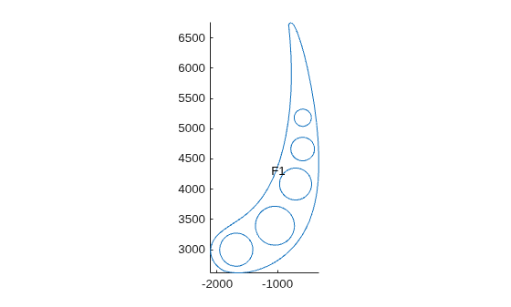

Fill the void regions with faces and plot the resulting geometry.

g = addFace(g,{3, 4, 5, 6, 7});

figure
pdegplot(g,FaceLabels="on")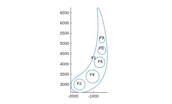

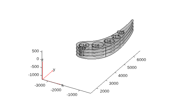
Extrude the geometry to create a stacked multilayer 3-D model of the blade. The thickness of each layer is 200 mm.

g = extrude(g,[200 200 200]);

Plot the geometry with the cell labels.

figure
pdegplot(g,CellLabels="on",FaceAlpha=0.5)