Clamped Square Isotropic Plate with Uniform Pressure Load

This example shows how to calculate the deflection of a structural plate under a pressure loading.

The partial differential equation for a thin isotropic plate with a pressure loading is

where $$D$$ is the bending stiffness of the plate given by

and $$E$$ is the modulus of elasticity, $$\nu$$ is Poisson's ratio, $$h$$ is the plate thickness, $$w$$ is the transverse deflection of the plate, and $$p$$ is the pressure load.

The boundary conditions for the clamped boundaries are $$w=0$$ and $$w^{\prime }=0$$, where $$w^{\prime }$$ is the derivative of $$w$$ in a direction normal to the boundary.

Partial Differential Equation Toolbox™ cannot directly solve this fourth-order plate equation. Convert the fourth-order equation to these two second-order partial differential equations, where $$v$$ is the new dependent variable.

You cannot directly specify boundary conditions for both $$w$$ and $$w^{\prime }$$ in this second-order system. Instead, specify that $$w^{\prime }$$ is 0, and define $$v^{\prime }$$ so that $$w$$ also equals 0 on the boundary. To specify these conditions, use stiff "springs" distributed along the boundary. The springs apply a transverse shear force to the plate edge. Define the shear force along the boundary due to these springs as $$n\cdot D\nabla v=-kw$$, where $$n$$ is the normal to the boundary, and $$k$$ is the stiffness of the springs. This expression is a generalized Neumann boundary condition supported by the toolbox. The value of $$k$$ must be large enough so that $$w$$ is approximately 0 at all points on the boundary. It also must be small enough to avoid numerical errors due to an ill-conditioned stiffness matrix.

The toolbox uses the dependent variables ${\mathit{u}}_1$ and ${\mathit{u}}_2$ instead of $$w$$ and $$v$$. Rewrite the two second-order partial differential equations using variables ${\mathit{u}}_1$ and ${\mathit{u}}_2$:

Create a PDE model for a system of two equations.

model = createpde(2);

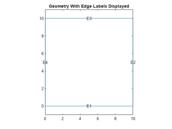
Create a square geometry and include it in the model.

len = 10;
gdm = [3 4 0 len len 0 0 0 len len]';
g = decsg(gdm,'S1',('S1')');
geometryFromEdges(model,g);

Plot the geometry with the edge labels.

figure
pdegplot(model,EdgeLabels="on")
xlim([-1,11])
ylim([-1,11])
title("Geometry With Edge Labels Displayed")

PDE coefficients must be specified using the format required by the toolbox. For details, see

The c coefficient in this example is a tensor, which can be represented as a 2-by-2 matrix of 2-by-2 blocks:

This matrix is further flattened into a column vector of six elements. The entries in the full 2-by-2 matrix (defining the coefficient a) and the 2-by-1 vector (defining the coefficient f) follow directly from the definition of the two-equation system.

E = 1.0e6; % Modulus of elasticity
nu = 0.3; % Poisson's ratio
thick = 0.1; % Plate thickness
pres = 2; % External pressure

D = E*thick^3/(12*(1 - nu^2));

c = [1 0 1 D 0 D]';
a = [0 0 1 0]';
f = [0 pres]';
specifyCoefficients(model,m=0,d=0,c=c,a=a,f=f);

To define boundary conditions, first specify spring stiffness.

k = 1e7;

Define distributed springs on all four edges.

bOuter = applyBoundaryCondition(model,"neumann",Edge=(1:4),...
                                g=[0 0],q=[0 0; k 0]);

Generate a mesh.

generateMesh(model);

Solve the model.

res = solvepde(model);

Access the solution at the nodal locations.

u = res.NodalSolution;

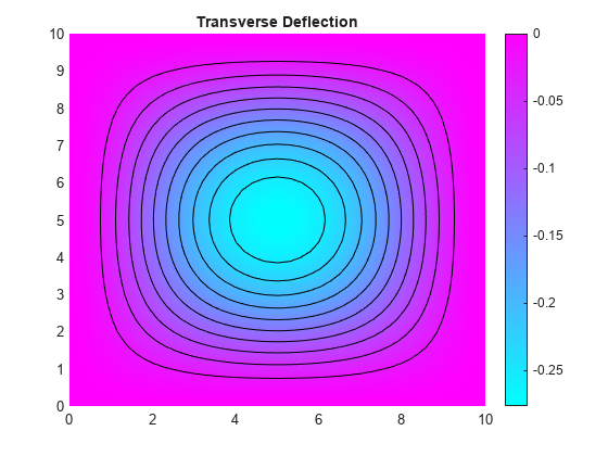
Plot the transverse deflection.

pdeplot(model,XYData=u(:,1),Contour="on")
title("Transverse Deflection")

Find the transverse deflection at the plate center.

numNodes = size(model.Mesh.Nodes,2);
wMax = min(u(1:numNodes,1))

wMax = 
-0.2762

Compare the result with the deflection at the plate center computed analytically.

wMax_exact = -.0138*pres*len^4/(E*thick^3)

wMax_exact = 
-0.2760