Solve PDEs with Constant Boundary Conditions

Open Live Script

This example shows how to apply various constant boundary condition specifications for both scalar PDEs and systems of PDEs.

Geometry

All the specifications use the same 2-D geometry, which is a rectangle with a circular hole.

% Rectangle is code 3, 4 sides,
% followed by x-coordinates and then y-coordinates
R1 = [3,4,-1,1,1,-1,-.4,-.4,.4,.4]';
% Circle is code 1, center (.5,0), radius .2
C1 = [1,.5,0,.2]';
% Pad C1 with zeros to enable concatenation with R1
C1 = [C1;zeros(length(R1)-length(C1),1)];
geom = [R1,C1];

% Names for the two geometric objects
ns = (char('R1','C1'))';

% Set formula
sf = 'R1 - C1';

% Create geometry
g = decsg(geom,sf,ns);

% Create geometry model
model = createpde;

% Include the geometry in the model
% and view the geometry
geometryFromEdges(model,g);
pdegplot(model,EdgeLabels="on")
xlim([-1.1 1.1])
axis equal

Figure contains an axes object. The axes object contains 9 objects of type line, text.

Scalar Problem

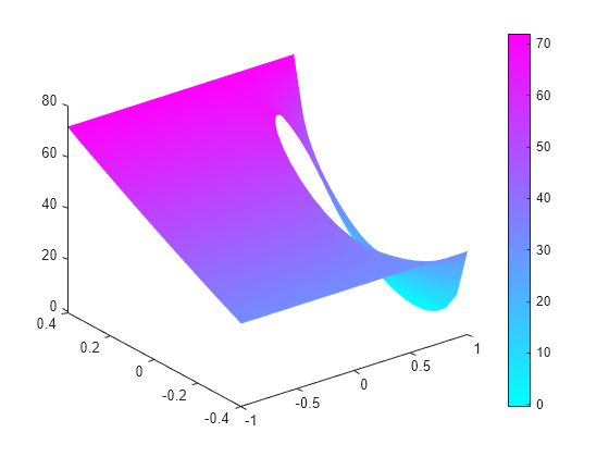
Suppose that edge 3 has Dirichlet conditions with value 32, edge 1 has Dirichlet conditions with value 72, and all other edges have Neumann boundary conditions with q = 0, g = -1.

applyBoundaryCondition(model,"dirichlet", ...
                       Edge=3,u=32);
applyBoundaryCondition(model,"dirichlet", ...
                       Edge=1,u=72);
applyBoundaryCondition(model,"neumann", ...
                       Edge=[2,4:8],g=-1);

This completes the boundary condition specification.

Solve an elliptic PDE with these boundary conditions with c = 1, a = 0, and f = 10. Because the shorter rectangular side has length 0.8, to ensure that the mesh is not too coarse choose a maximum mesh size Hmax = 0.1.

specifyCoefficients(model,m=0,d=0,c=1,a=0,f=10);
generateMesh(model,Hmax=0.1);
results = solvepde(model);
u = results.NodalSolution;
pdeplot(model,XYData=u,ZData=u)
view(-23,8)

Figure contains an axes object. The axes object contains an object of type patch.

System of PDEs

Suppose that the system has N = 2.

Edge 3 has Dirichlet conditions with values [32,72].
Edge 1 has Dirichlet conditions with values [72,32].
Edge 4 has a Dirichlet condition for the first component with value 52, and has a Neumann condition for the second component with q = 0, g = -1.
Edge 2 has Neumann boundary conditions with q = [1,2;3,4] and g = [5,-6].
The circular edges (edges 5 through 8) have q = 0 and g = 0.

model = createpde(2);
geometryFromEdges(model,g);

applyBoundaryCondition(model,"dirichlet", ...
                       Edge=3,u=[32,72]);
applyBoundaryCondition(model,"dirichlet", ...
                       Edge=1,u=[72,32]);
applyBoundaryCondition(model,"mixed", ...
                       Edge=4,u=52, ...
                       EquationIndex=1,g=[0,-1]);
Q2 = [1,2;3,4];
G2 = [5,-6];
applyBoundaryCondition(model,"neumann", ...
                       Edge=2,q=Q2,g=G2);

% The next step is optional,
% because it sets "g" to its default value
applyBoundaryCondition(model,"neumann", ...
                       Edge=5:8,g=[0,0]);