Contour Slices Through 3-D Solution with MATLAB Functions

Set Up and Solve the PDE

The problem is to solve Poisson's equation with zero Dirichlet boundary conditions for a complicated geometry. Poisson's equation is

Partial Differential Equation Toolbox™ solves equations in the form

So you can represent the problem by setting $$c=1$$ and $$a=0$$. Arbitrarily set $$f=10$$.

c = 1;
a = 0;
f = 10;

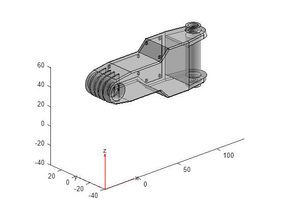
The first step in solving any 3-D PDE problem is to create a PDE Model. This is a container that holds the number of equations, geometry, mesh, and boundary conditions for your PDE. Create the model, then import the "ForearmLink.stl" file and view the geometry.

N = 1;
model = createpde(N);
importGeometry(model,"ForearmLink.stl");
pdegplot(model,FaceAlpha=0.5)
view(-42,24)

Specify PDE Coefficients

Include the PDE coefficients in model.

specifyCoefficients(model,m=0,d=0,c=c,a=a,f=f);

Create zero Dirichlet boundary conditions on all faces.

applyBoundaryCondition(model,"dirichlet", ...
                       Face=1:model.Geometry.NumFaces, ...
                       u=0);

Create a mesh and solve the PDE.

generateMesh(model);
result = solvepde(model);

Plot the Solution as Contour Slices

Because the boundary conditions are $$u=0$$ on all faces, the solution $$u$$ is nonzero only in the interior. To examine the interior, take a rectangular grid that covers the geometry with a spacing of one unit in each coordinate direction.

[X,Y,Z] = meshgrid(0:135,0:35,0:61);

For plotting and analysis, create a PDEResults object from the solution. Interpolate the result at every grid point.

V = interpolateSolution(result,X,Y,Z);
V = reshape(V,size(X));

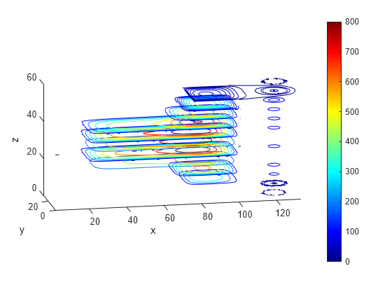
Plot contour slices for various values of $$z$$.

figure
colormap jet
contourslice(X,Y,Z,V,[],[],0:5:60)
xlabel("x")
ylabel("y")
zlabel("z")
colorbar
view(-11,14)
axis equal

Plot contour slices for various values of $$y$$.

figure
colormap jet
contourslice(X,Y,Z,V,[],1:6:31,[])
xlabel("x")
ylabel("y")
zlabel("z")
colorbar
view(-62,34)
axis equal

Save Memory by Evaluating As Needed

For large problems you can run out of memory when creating a fine 3-D grid. Furthermore, it can be time-consuming to evaluate the solution on a full grid. To save memory and time, evaluate only at the points you plot. You can also use this technique to interpolate to tilted grids, or to other surfaces.

For example, interpolate the solution to a grid on the tilted plane $$0\le x\le 135$$, $$0\le y\le 35$$, and $$z=x/10+y/2$$. Plot both contours and colored surface data. Use a fine grid, with spacing 0.2.

[X,Y] = meshgrid(0:0.2:135,0:0.2:35);
Z = X/10 + Y/2;
V = interpolateSolution(result,X,Y,Z);
V = reshape(V,size(X));
figure
subplot(2,1,1)
contour(X,Y,V);
axis equal
title("Contour Plot on Tilted Plane")
xlabel("x")
ylabel("y")
colorbar
subplot(2,1,2)
surf(X,Y,V,"LineStyle","none");
axis equal
view(0,90)
title("Colored Plot on Tilted Plane")
xlabel("x")
ylabel("y")
colorbar