Current Density Between Two Metallic Conductors: PDE Modeler App

Two circular metallic conductors are placed on a brine-soaked blotting paper which serves as a plane, thin conductor. The physical model for this problem consists of the Laplace equation

–∇ · (σ∇V) = 0

for the electric potential V and these boundary conditions:

V = 1 on the left circular conductor
V = –1 on the right circular conductor
the natural Neumann boundary condition on the outer boundaries
$\frac{\partial V}{\partial n} = 0$

The conductivity is σ = 1.

To solve this equation in the PDE Modeler app, follow these steps:

Model the geometry: draw the rectangle with corners at (-1.2,-0.6), (1.2,-0.6), (1.2,0.6), and (-1.2,0.6), and two circles with a radius of 0.3 and centers at (-0.6,0) and (0.6,0). The rectangle represents the blotting paper, and the circles represent the conductors.
```
pderect([-1.2 1.2 -0.6 0.6])
pdecirc(-0.6,0,0.3)
pdecirc(0.6,0,0.3)
```
Model the geometry by entering R1-(C1+C2) in the Set formula field.
Set the application mode to Conductive Media DC.
Specify the boundary conditions. To do this, switch to the boundary mode by selecting Boundary > Boundary Mode. Use Shift+click to select several boundaries. Then select Boundary > Specify Boundary Conditions.
- For the rectangle, use the Neumann boundary condition with g = 0 and q = 0.
- For the left circle, use the Dirichlet boundary condition with h = 1 and r = 1.
- For the right circle, use the Dirichlet boundary condition with h = 1 and r = -1.
Specify the coefficients by selecting PDE > PDE Specification or clicking the button on the toolbar. Specify sigma = 1 and q = 0.
Initialize the mesh by selecting Mesh > Initialize Mesh.
Refine the mesh by selecting Mesh > Refine Mesh.
Improve the triangle quality by selecting Mesh > Jiggle Mesh.
Solve the PDE by selecting Solve > Solve PDE or clicking the button on the toolbar. The resulting potential is zero along the y-axis, which, for this problem, is a vertical line of antisymmetry.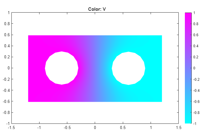
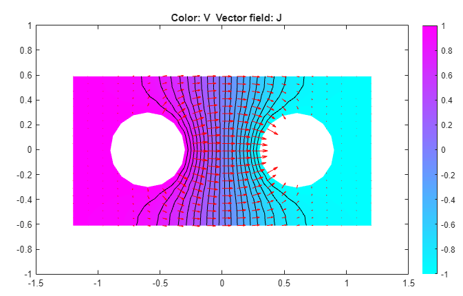
Plot the current density J. To do this:
1. Select Plot > Parameters.
2. In the resulting dialog box, select the Color, Contour, and Arrows options.
3. Set the Arrows value to current density.
The current flows, as expected, from the conductor with a positive potential to the conductor with a negative potential. The conductivity σ is isotropic, and the equipotential lines are orthogonal to the current lines.

Current Density Between Two Metallic Conductors: PDE Modeler App

WeChat