Deflection of Piezoelectric Actuator

This example shows how to solve a coupled elasticity-electrostatics problem.

Piezoelectric materials deform under an applied voltage. Conversely, deforming a piezoelectric material produces a voltage. Therefore, analysis of a piezoelectric part requires the solution of a set of coupled partial differential equations with deflections and electrical potential as dependent variables.

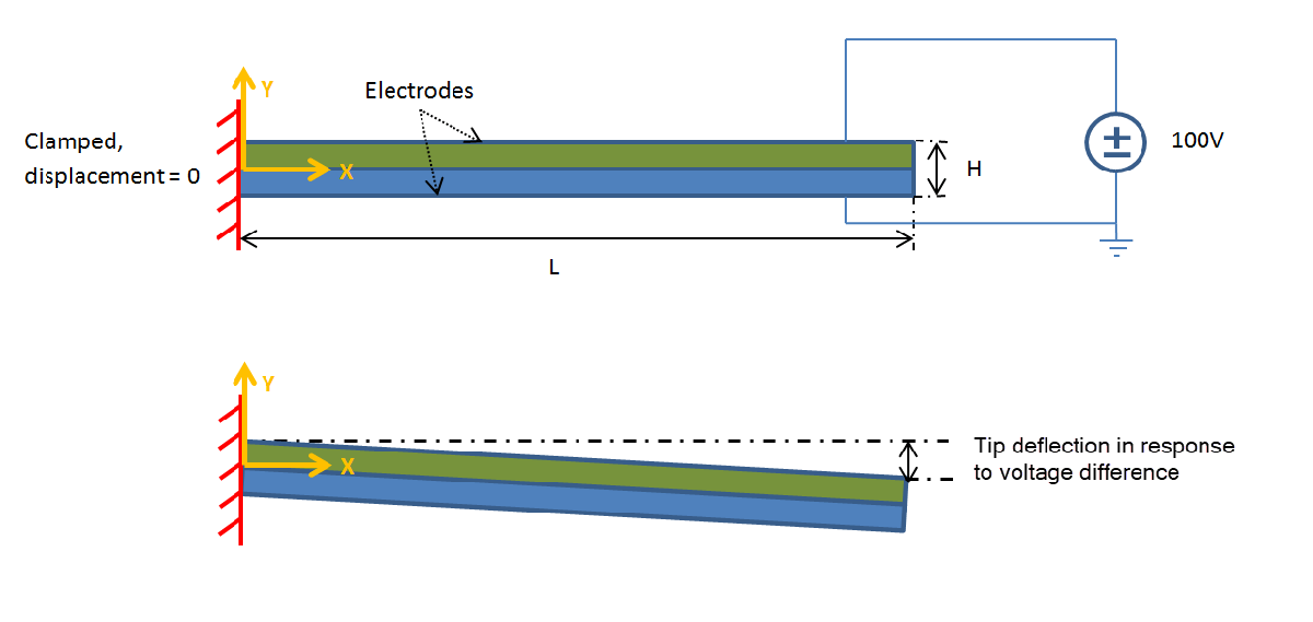
In this example, the model is a two-layer cantilever beam, with both layers made of the same polyvinylidene fluoride (PVDF) material. The polarization direction points down (negative y-direction) in the top layer and points up in the bottom layer. The typical length to thickness ratio is 100. When you apply a voltage between the lower and upper surfaces of the beam, the beam deflects in the y-direction because one layer shortens and the other layer lengthens.

Clamped cantilever beam with a voltage applied between the lower and upper surfaces. First, the beam is shown without the tip deflection. Then, it is shown with the tip deflection in response to voltage difference.

The equilibrium equations describe the elastic behavior of the solid:

$- \nabla \cdot σ = f$

Here, $σ$ is the stress tensor, and $f$ is the body force vector. Gauss's Law describes the electrostatic behavior of the solid:

$\nabla \cdot D = ρ$

$D$ is the electric displacement, and $ρ$ is the distributed free charge. Combine these two PDE systems into this single system:

$- \nabla \cdot {\begin{array}{c} σ \\ D \end{array}} = {\begin{array}{c} f \\ - ρ \end{array}}$

For a 2-D analysis, $σ$ has the components $σ_{11}, σ_{22},$ and $σ_{12} = σ_{21}$ , and $D$ has the components $D_{1}$ and $D_{2}$ .

The constitutive equations for the material define the stress tensor and electric displacement vector in terms of the strain tensor and electric field. For a 2-D analysis of an orthotropic piezoelectric material under plane stress conditions, you can write these equations as

${\begin{array}{c} σ_{11} \\ σ_{22} \\ σ_{12} \\ D_{1} \\ D_{2} \end{array}} = [\begin{array}{ccccc} C_{11} & C_{12} & e_{11} & e_{31} \\ C_{12} & C_{22} & e_{13} & e_{33} \\ G_{12} & e_{14} & e_{34} \\ e_{11} & e_{13} & e_{14} & - E_{1} \\ e_{31} & e_{33} & e_{34} & - E_{2} \end{array}] {\begin{array}{c} ϵ_{11} \\ ϵ_{22} \\ γ_{12} \\ - E_{1} \\ - E_{2} \end{array}}$

$C_{i j}$ are the elastic coefficients, $E_{i}$ are the electrical permittivities, and $e_{i j}$ are the piezoelectric stress coefficients. The piezoelectric stress coefficients in these equations conform to conventional notation in piezoelectric materials where the z-direction (the third direction) aligns with the "poled" direction of the material. For the 2-D analysis, align the "poled" direction with the y-axis. Write the strain vector in terms of the x-displacement $u$ and y-displacement $v$ :

${\begin{array}{c} ϵ_{11} \\ ϵ_{22} \\ γ_{12} \end{array}} = {\begin{array}{c} \frac{\partial u}{\partial x} \\ \frac{\partial v}{\partial y} \\ \frac{\partial u}{\partial y} + \frac{\partial v}{\partial x} \end{array}}$

Write the electric field in terms of the electrical potential $ϕ$ :

${\begin{array}{c} E_{1} \\ E_{2} \end{array}} = - {\begin{array}{c} \frac{\partial ϕ}{\partial x} \\ \frac{\partial ϕ}{\partial y} \end{array}}$

You can substitute the strain-displacement equations and electric field equations into the constitutive equations and get a system of equations for the stresses and electrical displacements in terms of displacement and electrical potential derivatives. Substituting the resulting equations into the PDE system equations yields a system of equations that involve the divergence of the displacement and electrical potential derivatives. As the next step, arrange these equations to match the form required by the toolbox.

Partial Differential Equation Toolbox™ requires a system of elliptic equations to be expressed in a vector form:

$- \nabla \cdot (c \otimes \nabla u) + a u = f$

or in a tensor form:

$- \frac{\partial}{\partial x_{k}} (c_{i j k l} \frac{\partial u_{j}}{\partial x_{l}}) + a_{i j} u_{j} = f_{i}$

where repeated indices imply summation. For the 2-D piezoelectric system in this example, the system vector $u$ is

$u = {\begin{array}{c} u \\ v \\ ϕ \end{array}}$

This is an $N = 3$ system. The gradient of $u$ is

$\nabla u = {\begin{array}{c} \frac{\partial u}{\partial x} \\ \frac{\partial u}{\partial y} \\ \frac{\partial v}{\partial x} \\ \frac{\partial v}{\partial y} \\ \frac{\partial ϕ}{\partial x} \\ \frac{\partial ϕ}{\partial y} \end{array}}$

For details on specifying the coefficients in the format required by the toolbox, see:

The c coefficient in this example is a tensor. You can represent it as a 3-by-3 matrix of 2-by-2 blocks:

$[\begin{array}{cccccc} c (1) & c (3) & c (13) & c (15) & c (25) & c (27) \\ c (2) & c (4) & c (14) & c (16) & c (26) & c (28) \\ с (5) & c (7) & c (17) & c (19) & c (29) & c (31) \\ c (6) & c (8) & с (18) & c (20) & c (30) & c (32) \\ с (9) & c (11) & с (21) & c (23) & c (33) & c (35) \\ с (10) & c (12) & с (22) & c (24) & c (34) & c (36) \end{array}]$

To map terms of constitutive equations to the form required by the toolbox, write the c tensor and the solution gradient in this form:

$[\begin{array}{cccccc} c_{1111} & c_{1112} & c_{1211} & c_{1212} & c_{1311} & c_{1312} \\ c_{1121} & c_{1122} & c_{1221} & c_{1222} & c_{1321} & c_{1322} \\ c_{2111} & c_{2112} & c_{2211} & c_{2212} & c_{2311} & c_{2312} \\ c_{2121} & c_{2122} & c_{2221} & c_{2222} & c_{2321} & c_{2322} \\ c_{3111} & c_{3112} & c_{3211} & c_{3212} & c_{3311} & c_{3312} \\ c_{3121} & c_{3122} & c_{3221} & c_{3222} & c_{3321} & c_{3322} \end{array}] {\begin{array}{c} \frac{\partial u}{\partial x} \\ \frac{\partial u}{\partial y} \\ \frac{\partial v}{\partial x} \\ \frac{\partial v}{\partial y} \\ \frac{\partial ϕ}{\partial x} \\ \frac{\partial ϕ}{\partial y} \end{array}}$

From this equation, you can map the traditional constitutive coefficients to the form required for the c matrix. The minus sign in the equations for the electric field is incorporated into the c matrix to match the toolbox's convention.

$[\begin{array}{cccccc} C_{11} & \cdot & \cdot & C_{12} & e_{11} & e_{31} \\ \cdot & G_{12} & G_{12} & \cdot & e_{14} & e_{34} \\ \cdot & G_{12} & G_{12} & \cdot & e_{14} & e_{34} \\ C_{21} & \cdot & \cdot & C_{22} & e_{13} & e_{33} \\ e_{11} & e_{14} & e_{14} & e_{13} & - E_{1} & \cdot \\ e_{31} & e_{34} & e_{34} & e_{33} & \cdot & - E_{2} \end{array}] {\begin{array}{c} \frac{\partial u}{\partial x} \\ \frac{\partial u}{\partial y} \\ \frac{\partial v}{\partial x} \\ \frac{\partial v}{\partial y} \\ \frac{\partial ϕ}{\partial x} \\ \frac{\partial ϕ}{\partial y} \end{array}}$

Beam Geometry

Create a PDE model. The equations have three components: two components due to linear elasticity and one component due to electrostatics. Therefore, the model must have three equations.

model = createpde(3);

Create the geometry and include it in the model.

L = 100e-3; % Beam length in meters
H = 1e-3; % Overall height of the beam
H2 = H/2; % Height of each layer in meters

topLayer = [3 4 0 L L 0 0 0 H2 H2];
bottomLayer = [3 4 0 L L 0 -H2 -H2 0 0];
gdm = [topLayer;bottomLayer]';
g = decsg(gdm,'R1+R2',['R1';'R2']');

geometryFromEdges(model,g);

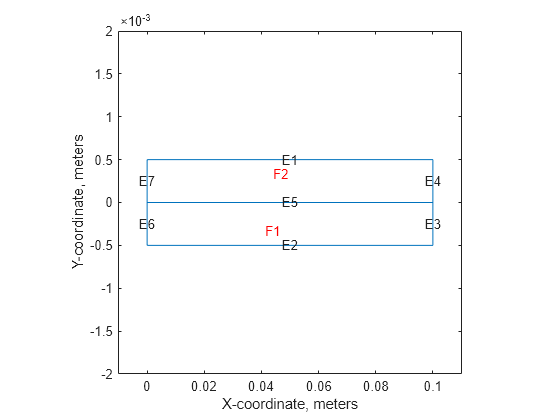
Plot the geometry with the face and edge labels.

figure
pdegplot(model,EdgeLabels="on", ...
               FaceLabels="on")
xlabel("X-coordinate, meters")
ylabel("Y-coordinate, meters")
axis([-.1*L,1.1*L,-4*H2,4*H2])
axis square

Figure contains an axes object. The axes object with xlabel X-coordinate, meters, ylabel Y-coordinate, meters contains 10 objects of type line, text.

Material Properties

Specify the material properties of the beam layers. The material in both layers is polyvinylidene fluoride (PVDF), a thermoplastic polymer with piezoelectric behavior.

E = 2.0e9; % Elastic modulus, N/m^2
NU = 0.29; % Poisson's ratio
G = 0.775e9; % Shear modulus, N/m^2
d31 = 2.2e-11; % Piezoelectric strain coefficients, C/N
d33 = -3.0e-11;

Specify relative electrical permittivity of the material at constant stress.

relPermittivity = 12;

Specify the electrical permittivity of vacuum.

permittivityFreeSpace = 8.854187817620e-12; % F/m
C11 = E/(1 - NU^2); 
C12 = NU*C11;
c2d = [C11 C12 0; C12 C11 0; 0 0 G];
pzeD = [0 d31; 0 d33; 0 0];

Specify the piezoelectric stress coefficients.

pzeE = c2d*pzeD;
D_const_stress = [relPermittivity 0;
                  0 relPermittivity]*permittivityFreeSpace;

Convert the dielectric matrix from constant stress to constant strain.

D_const_strain = D_const_stress - pzeD'*pzeE;

The parameters of the elastic equations are of the order of $10^{9}$ while the electric parameters are of the order of $10^{- 11} .$ To avoid constructing an ill-conditioned matrix, rescale the last equation so that the coefficients are larger. Note that before any post-processing involving the c coefficient (for example, when you evaluate a flux of PDE solution), you must revert the scaling changes to the c matrix.

cond_scaling = 1e5;

You can view the 36 coefficients as a 3-by-3 matrix of 2-by-2 blocks.

c11 = [c2d(1,1) c2d(1,3) c2d(3,1) c2d(3,3)];
c12 = [c2d(1,3) c2d(1,2); c2d(3,3) c2d(2,3)];
c21 = c12';

c22 = [c2d(3,3) c2d(2,3) c2d(3,2) c2d(2,2)];
c13 = [pzeE(1,1) pzeE(1,2); pzeE(3,1) pzeE(3,2)];
c31 = cond_scaling*c13';
c23 = [pzeE(3,1) pzeE(3,2); pzeE(2,1) pzeE(2,2)];
c32 = cond_scaling*c23';

c33 = cond_scaling*[D_const_strain(1,1)
                    D_const_strain(2,1)
                    D_const_strain(1,2)
                    D_const_strain(2,2)];
ctop = [c11(:); c21(:); -c31(:);
        c12(:); c22(:); -c32(:);
       -c13(:); -c23(:); -c33(:)];
cbot = [c11(:); c21(:); c31(:);
        c12(:); c22(:); c32(:);
        c13(:); c23(:); -c33(:)];

If you problem includes a current source for the third equation, scale the f coefficient: f = [0 0 cond_scaling*value_f]'. Otherwise, specify it as follows.

f = [0 0 0]';

Specify coefficients.

specifyCoefficients(model,m=0,d=0,c=ctop,a=0,f=f,Face=2);
specifyCoefficients(model,m=0,d=0,c=cbot,a=0,f=f,Face=1);

Boundary Conditions

Set the voltage (solution component 3) on the top of the beam (edge 1) to 100 volts.

voltTop = ...
    applyBoundaryCondition(model,"mixed", ...
                           Edge=1,u=100,...
                           EquationIndex=3);

Specify that the bottom of the beam (edge 2) is grounded by setting the voltage to 0.

voltBot = ...
    applyBoundaryCondition(model,"mixed", ...
                           Edge=2,...
                           u=0,...
                           EquationIndex=3);

Specify that the left side (edges 6 and 7) is clamped by setting the x- and y-displacements (solution components 1 and 2) to 0.

clampLeft = ...
    applyBoundaryCondition(model,"mixed", ...
                           Edge=6:7,...
                           u=[0 0],...
                           EquationIndex=1:2);

The stress and charge on the right side of the beam are zero. Accordingly, use the default boundary condition for edges 3 and 4.

Finite Element and Analytical Solutions

Generate a mesh and solve the model.

msh = generateMesh(model,Hmax=5e-4);
result = solvepde(model)

result = 
  StationaryResults with properties:

    NodalSolution: [3605x3 double]
       XGradients: [3605x3 double]
       YGradients: [3605x3 double]
       ZGradients: [0x3 double]
             Mesh: [1x1 FEMesh]

Access the solution at the nodal locations. The first column contains the x-deflection. The second column contains the y-deflection. The third column contains the electrical potential.

rs = result.NodalSolution;

Find the minimum y-deflection.

feTipDeflection = min(rs(:,2));
fprintf("Finite element tip deflection is: %12.4e\n",feTipDeflection);

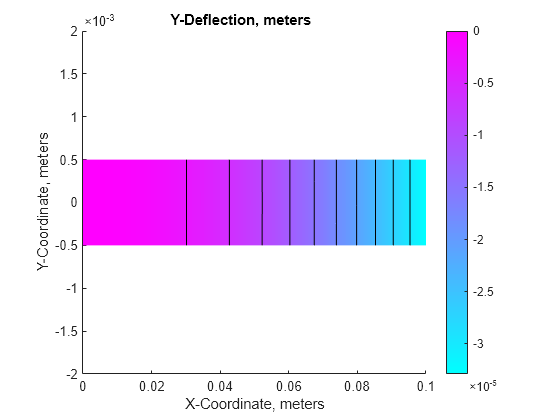
Finite element tip deflection is:  -3.2900e-05

Compare this result with the known analytical solution.

tipDeflection = -3*d31*100*L^2/(8*H2^2);
fprintf("Analytical tip deflection is: %12.4e\n",tipDeflection);

Analytical tip deflection is:  -3.3000e-05

Plot the deflection components and the electrical potential.

varsToPlot = char('X-Deflection, meters', ...
                  'Y-Deflection, meters', ...
                  'Electrical Potential, Volts');
for i = 1:size(varsToPlot,1)
  figure;
  pdeplot(model,XYData=rs(:,i),Contour="on")
  title(varsToPlot(i,:))
  % scale the axes to make it easier to view the contours
  axis([0, L, -4*H2, 4*H2])
  xlabel("X-Coordinate, meters")
  ylabel("Y-Coordinate, meters")
  axis square
end

Figure contains an axes object. The axes object with title X-Deflection, meters, xlabel X-Coordinate, meters, ylabel Y-Coordinate, meters contains 12 objects of type patch, line.

Figure contains an axes object. The axes object with title Y-Deflection, meters, xlabel X-Coordinate, meters, ylabel Y-Coordinate, meters contains 12 objects of type patch, line.

Figure contains an axes object. The axes object with title Electrical Potential, Volts, xlabel X-Coordinate, meters, ylabel Y-Coordinate, meters contains 12 objects of type patch, line.

References

Hwang, Woo-Seok, and Hyun Chul Park. "Finite Element Modeling of Piezoelectric Sensors and Actuators." AIAA Journal 31, no.5 (May 1993): 930-937.
Pieford, V. "Finite Element Modeling of Piezoelectric Active Structures." PhD diss., Universite Libre De Bruxelles, 2001.