Heat Transfer Problem with Temperature-Dependent Properties

Steady-State Solution: Constant Thermal Conductivity

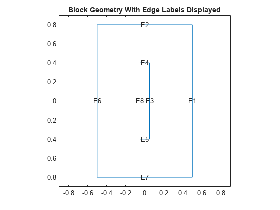
Create a 2-D geometry by drawing one rectangle the size of the block and a second rectangle the size of the slot.

r1 = [3 4 -.5 .5 .5 -.5 -.8 -.8 .8 .8];
r2 = [3 4 -.05 .05 .05 -.05 -.4 -.4 .4 .4];
gdm = [r1; r2]';

Subtract the second rectangle from the first to create the block with a slot.

g = decsg(gdm,'R1-R2',['R1'; 'R2']');

Plot the geometry with edge labels displayed. The edge labels will be used below in the function for defining boundary conditions.

figure
pdegplot(g,EdgeLabels="on"); 
axis([-.9 .9 -.9 .9]);
title("Block Geometry With Edge Labels Displayed")

Create an femodel object for steady-state thermal analysis and include the geometry in the model.

model = femodel(AnalysisType="thermalSteady", ...
                Geometry=g);

Set the temperature on the left edge to 100 degrees.

model.EdgeBC(4) = edgeBC(Temperature=100);

On the right edge, there is a prescribed heat flux out of the block

model.EdgeLoad(2) = edgeLoad(Heat=-10);

The top and bottom edges and the edges inside the cavity are all insulated, that is, no heat is transferred across these edges.

Specify the thermal conductivity of the material. First, consider the constant thermal conductivity, for example, equal one. Later, consider a case where the thermal conductivity is a function of temperature.

model.MaterialProperties = ...
    materialProperties(ThermalConductivity=1);

Create a mesh with elements no larger than 0.2.

model = generateMesh(model,Hmax=0.2);
figure 
pdemesh(model); 
axis equal
title("Block With Finite Element Mesh Displayed")

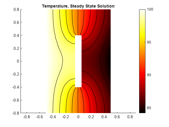
Calculate the steady-state solution.

R = solve(model);
T = R.Temperature;
figure
pdeplot(R.Mesh,XYData=T,Contour="on",ColorMap="hot"); 
axis equal
title("Temperature, Steady State Solution")

Transient Solution: Constant Thermal Conductivity

Switch the analysis type of the model to transient thermal analysis.

model.AnalysisType = "thermalTransient";

Specify mass density and specific heat of the material.

model.MaterialProperties.MassDensity = 1;
model.MaterialProperties.SpecificHeat = 1;

Define boundary conditions. In the transient cases, the temperature on the left edge is zero at time=0 and ramps to 100 degrees over .5 seconds. You can find the helper function transientBCHeatedBlock under matlab/R20XXx/examples/pde/main.

model.EdgeBC(4) = ...
    edgeBC(Temperature=@transientBCHeatedBlock);

Calculate the transient solution. Perform a transient analysis from zero to five seconds. The toolbox saves the solution every .1 seconds so that plots of the results as functions of time can be created.

tlist = 0:.1:5;
model.FaceIC = faceIC(Temperature=0);
R = solve(model,tlist);
T = R.Temperature;
msh = R.Mesh;

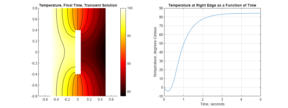
Two plots are useful in understanding the results from this transient analysis. The first is a plot of the temperature at the final time. The second is a plot of the temperature at a specific point in the block, in this case near the center of the right edge, as a function of time. To identify a node near the center of the right edge, it is convenient to define this short utility function.

getClosestNode = @(p,x,y) min((p(1,:) - x).^2 + (p(2,:) - y).^2);

Call this function to get a node near the center of the right edge.

[~,nid] = getClosestNode(msh.Nodes,.5,0);

The two plots are shown side-by-side in the figure below. The temperature distribution at this time is very similar to that obtained from the steady-state solution above. At the right edge, for times less than about one-half second, the temperature is less than zero. This is because heat is leaving the block faster than it is arriving from the left edge. At times greater than about three seconds, the temperature has essentially reached steady-state.

h = figure;
h.Position = [1 1 2 1].*h.Position;
subplot(1,2,1); 
axis equal
pdeplot(msh,XYData=T(:,end),Contour="on", ...
                            ColorMap="hot"); 
axis equal
title("Temperature, Final Time, Transient Solution")
subplot(1,2,2); 
axis equal
plot(tlist, T(nid,:)); 
grid on
title("Temperature at Right Edge as a Function of Time")
xlabel("Time, seconds")
ylabel("Temperature, degrees-Celsius")

Steady State Solution: Temperature-Dependent Thermal Conductivity

It is not uncommon for material properties to be functions of the dependent variables. For example, assume that the thermal conductivity is a simple linear function of temperature:

k = @(location,state) 0.3+0.003*state.u;

In this case, the variable u is the temperature. For this example, assume that the density and specific heat are not functions of temperature.

model.MaterialProperties.ThermalConductivity = k;

Switch the analysis type of the model to steadystate thermal analysis.

model.AnalysisType = "thermalSteady";

Set the temperature on the left edge to 100 degrees.

model.EdgeBC(4) = edgeBC(Temperature=100);

Calculate the steady-state solution. Compared with the constant-conductivity case, the temperature on the right-hand edge is lower. This is due to the lower conductivity in regions with lower temperature.

R = solve(model);
T = R.Temperature;
msh = R.Mesh;
figure
pdeplot(msh,XYData=T,Contour="on",ColorMap="hot");  
axis equal
title("Temperature, Steady State Solution")

Transient Solution: Temperature-Dependent Thermal Conductivity

Now perform a transient analysis with the temperature-dependent conductivity.

model.AnalysisType = "thermalTransient";
model.EdgeBC(4) = edgeBC(Temperature=@transientBCHeatedBlock);

Use the same timespan tlist = 0:.1:5 as for the linear case.

R = solve(model,tlist);
T = R.Temperature;
msh = R.Mesh;

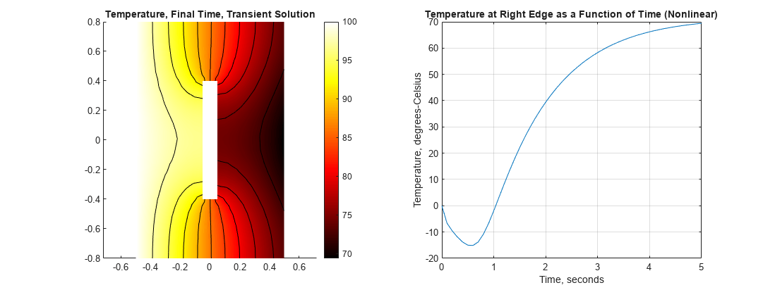
Plot the temperature at the final time step and the temperature at the right edge as a function of time. The plot of temperature at the final time step is only slightly different from the comparable plot from the linear analysis: temperature at the right edge is slightly lower than the linear case. The plot of temperature as a function of time is considerably different from the linear case. Because of the lower conductivity at lower temperatures, the heat takes longer to reach the right edge of the block. In the linear case, the temperature is essentially constant at around three seconds but for this nonlinear case, the temperature curve is just beginning to flatten at five seconds.

h = figure;
h.Position = [1 1 2 1].*h.Position;
subplot(1,2,1); 
axis equal
pdeplot(msh,XYData=T(:,end),Contour="on", ...
                            ColorMap="hot"); 
axis equal
title("Temperature, Final Time, Transient Solution")
subplot(1,2,2); 
axis equal
plot(tlist(1:size(T,2)), T(nid,:)); 
grid on
title("Temperature at Right Edge as a Function of Time (Nonlinear)")
xlabel("Time, seconds")
ylabel("Temperature, degrees-Celsius")