Inhomogeneous Heat Equation on Square Domain
This example shows how to solve the heat equation with a source term.
The basic heat equation with a unit source term is
This equation is solved on a square domain with a discontinuous initial condition and zero temperatures on the boundaries.
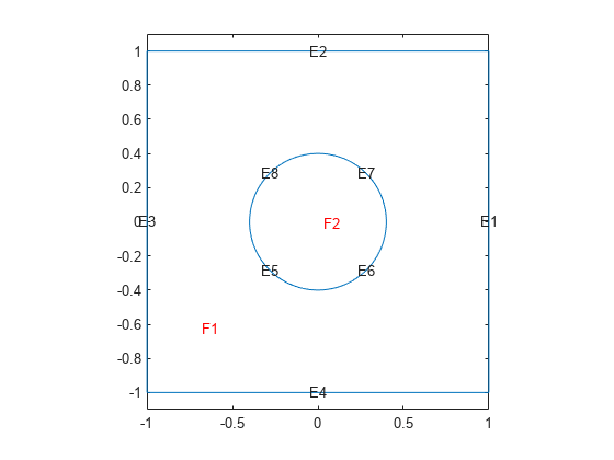
Create a square geometry centered at x = 0 and y = 0 with sides of length 2. Include a circle of radius 0.4 concentric with the square.
R1 = [3;4;-1;1;1;-1;-1;-1;1;1];
C1 = [1;0;0;0.4];
C1 = [C1;zeros(length(R1) - length(C1),1)];
gd = [R1,C1];
sf = 'R1+C1';
ns = char('R1','C1')';
g = decsg(gd,sf,ns);
Plot the geometry with edge and face labels.
figure
pdegplot(g,EdgeLabels="on",FaceLabels="on")
axis([-1.1 1.1 -1.1 1.1]);
axis equal

Create an femodel object for transient thermal analysis and include the geometry.
model = femodel(AnalysisType="thermalTransient", ...
                Geometry=g);
Specify thermal properties of the material.
model.MaterialProperties = ...
    materialProperties(ThermalConductivity=1,...
                       MassDensity=1,...
                       SpecificHeat=1);
Specify internal heat source.
model.FaceLoad = faceLoad(Heat=1);
Set zero temperatures on all four outer edges of the square.
model.EdgeBC(1:4) = edgeBC(Temperature=0);
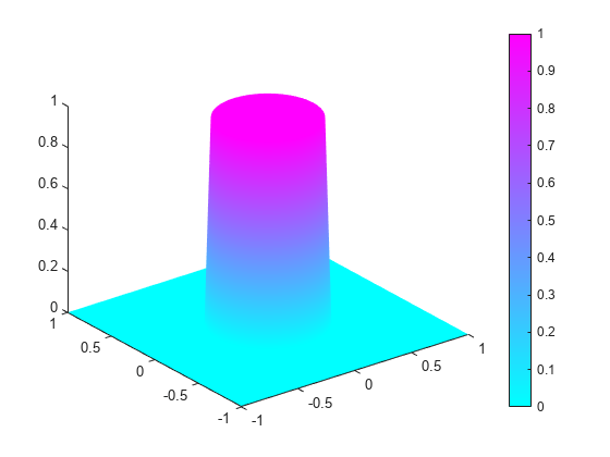
The discontinuous initial value is 1 inside the circle and zero outside. Specify zero initial temperature everywhere.
model.FaceIC = faceIC(Temperature=0);
Specify nonzero initial temperature inside the circle (Face 2).
model.FaceIC(2) = faceIC(Temperature=1);
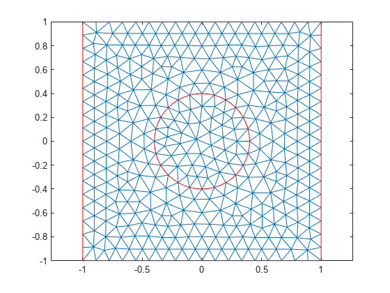
Generate and plot a mesh.
model = generateMesh(model);
figure;
pdemesh(model);
axis equal
Find the solution at 20 points in time between 0 and 0.1.
nframes = 20;
tlist = linspace(0,0.1,nframes);

model.SolverOptions.ReportStatistics ='on';
result = solve(model,tlist);
T = result.Temperature;
Plot the solution.
figure
Tmax = max(max(T));
Tmin = min(min(T));
for j = 1:nframes
    pdeplot(result.Mesh,XYData=T(:,j),ZData=T(:,j));
    axis([-1 1 -1 1 0 1]);
    Mv(j) = getframe;
end

To play the animation, use the movie(Mv,1) command.
