Nonlinear Magnetic Permeability from B-H Curve

Open Live Script

This example shows how to solve a 2-D nonlinear magnetostatic problem for a ferromagnetic frame with an H-shaped cavity. This setup generates a magnetic field due to the presence of two coils. First, calculate a solution using constant relative permeability. Then use the results as an initial guess for a nonlinear magnetostatic model, with the relative permeability depending on the magnetic flux density.

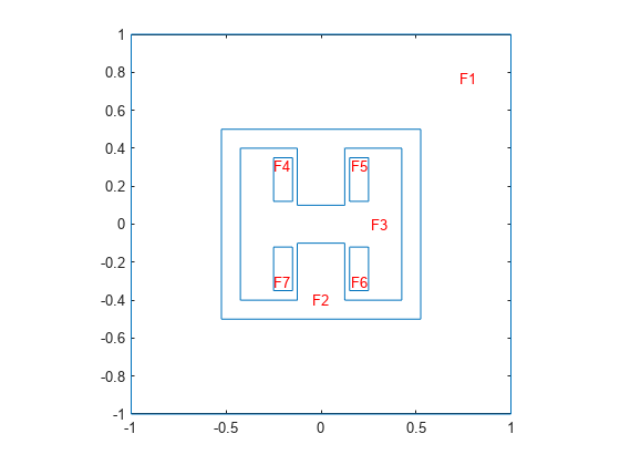
Create a geometry that consists of a rectangular frame with an H-shaped cavity, four rectangles representing the two coils, and a unit square representing the air domain around the magnet. Specify all dimensions in millimeters, and use the value 1000 to convert the dimensions to meters.

convfactor = 1000;

First, create the H-shaped geometry to model the cavity.

xCoordsCavity = [-425 -125 -125 125 125 425 425 ...
               125 125 -125 -125 -425]/convfactor;
yCoordsCavity = [-400 -400 -100 -100 -400 -400 ...
               400 400 100 100 400 400]/convfactor;
RH = [2;12;xCoordsCavity';yCoordsCavity'];

Create the geometry to model the rectangular ferromagnetic frame.

RS = [3;4;[-525;525;525;-525;-500;-500;500;500]/convfactor];
zeroPad  = zeros(numel(RH)-numel(RS),1);
RS = [RS;zeroPad];

Create the geometries to model the coils.

RC1 = [3;4;[150;250;250;150;120;120;350;350]/convfactor;
                                                zeroPad];
RC2 = [3;4;[-150;-250;-250;-150;120;120;350;350]/convfactor;
                                                zeroPad];
RC3 = [3;4;[150;250;250;150;-120;-120;-350;-350]/convfactor;
                                                zeroPad];
RC4 = [3;4;[-150;-250;-250;-150;-120;-120;-350;-350]/convfactor;
                                                zeroPad];

Create the geometry to model the air domain around the magnet.

RD = [3;4;[-1000;1000;1000;-1000;-1000; ...
           -1000;1000;1000]/convfactor;zeroPad];

Combine the shapes into one matrix.

gd = [RS,RH,RC1,RC2,RC3,RC4,RD];

Create a set formula and create the geometry.

ns = char('RS','RH','RC1','RC2','RC3','RC4','RD');
g = decsg(gd,'(RS+RH+RC1+RC2+RC3+RC4)+RD',ns');

Plot the geometry with face labels.

pdegplot(g,FaceLabels="on")

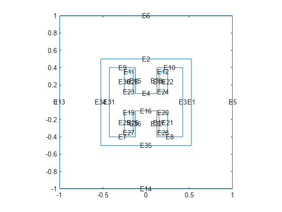
Figure contains an axes object. The axes object contains 8 objects of type line, text.

Plot the geometry with edge labels.

figure
pdegplot(g,EdgeLabels="on")

Figure contains an axes object. The axes object contains 37 objects of type line, text.

Create a magnetostatic model and include the geometry in the model.

model = femodel(AnalysisType="magnetostatic", ...
                Geometry=g);

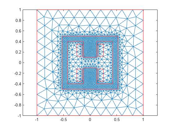
Generate a mesh with fine refinement in the ferromagnetic frame.

model = generateMesh(model,Hface={2,0.025}, ...
                           Hmax=0.2, ...
                           Hgrad=2);

Plot the mesh.

figure
pdemesh(model)

Figure contains an axes object. The axes object contains 2 objects of type line.

Specify the vacuum permeability value in the SI system of units.

mu0 = 1.25663706212e-6;
model.VacuumPermeability = mu0;

Specify a relative permeability of 1 for all domains.

model.MaterialProperties = materialProperties(RelativePermeability=1);

Now specify the large constant relative permeability of the ferromagnetic frame.

model.MaterialProperties(2) = ...
         materialProperties(RelativePermeability=10000);

Specify the current density values on the upper and lower coils.

model.FaceLoad([5 6]) = faceLoad(CurrentDensity=1e6);
model.FaceLoad([4 7]) = faceLoad(CurrentDensity=-1e6);

Specify that the magnetic potential on the outer surface of the air domain is 0.

model.EdgeBC([5 6 13 14]) = edgeBC(MagneticPotential=0);

Solve the linear magnetostatic model.

Rlin = solve(model)

Rlin = 
  MagnetostaticResults with properties:

      MagneticPotential: [6373x1 double]
          MagneticField: [1x1 FEStruct]
    MagneticFluxDensity: [1x1 FEStruct]
                   Mesh: [1x1 FEMesh]

Specify the data for the magnetic flux density B and the corresponding magnetic field strength H.

B = [0 .3 .8 1.12 1.32 1.46 1.54 1.61875 1.74];
H = [0 29.8 79.6 159.2 318.31 795.8 1591.6 3376.7 7957.8];

From the data for B and H, interpolate the H(B) dependency (B-H curve) using the modified Akima cubic Hermite interpolation method.

HofB = griddedInterpolant(B,H,"makima","linear");
muR = @(B) B./HofB(B)/mu0;

Specify the relative permeability of the ferromagnetic frame as a function of B, $μ_{R} = B / H$ .

model.MaterialProperties(2) =  ...
        materialProperties(RelativePermeability= ...
                           @(~,s) muR(s.NormFluxDensity));

Specify the initial guess by using the results obtained by the linear solver.

model.FaceIC = faceIC(MagneticVectorPotential=Rlin);

Solve the nonlinear magnetostatic model.

Rnonlin = solve(model);

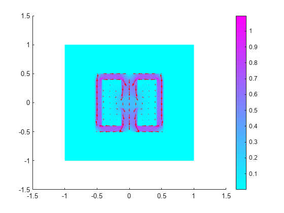
Plot the magnitude of the flux density.

Bmag = sqrt(Rnonlin.MagneticFluxDensity.Bx.^2 + ...
            Rnonlin.MagneticFluxDensity.By.^2);
figure
pdeplot(Rnonlin.Mesh,XYData=Bmag, ...
                     FlowData=[Rnonlin.MagneticFluxDensity.Bx ...
                               Rnonlin.MagneticFluxDensity.By])

Figure contains an axes object. The axes object contains 2 objects of type patch, quiver.

References

[1] Kozlowski, A., R. Rygal, and S. Zurek. "Large DC electromagnet for semi-industrial thermomagnetic processing of nanocrystalline ribbon." IEEE Transactions on Magnetics 50, issue 4 (April 2014): 1–4. https://ieeexplore.ieee.org/document/6798057.