Model Battery Performance
Simulate the battery discharge with a dynamic current profile and battery charging with a constant current. Incorporate the Arrhenius temperature correction on diffusion coefficients and ionic conductivity.
Specify the reference temperature for Arrhenius dependency of material properties and the simulation temperature, in K.
Tref = 296.15;
SimulationTemperature = Tref - 10;
Specify the universal gas constant, the Faraday constant, the Boltzmann constant, and the elementary charge.
R = 8.31446; % J/(mol·K))
FaradayConstant = 96487; % C/mol
BoltzmannConstant = 1.380649E-23; % J/K
ElementaryCharge = 1.6021766E-19; % C
Anode Properties
Specify the properties of the battery anode. First, create an object that specifies the active material of the anode, including the particle radius, maximum solid-phase concentration of lithium ions, fraction of the anode volume occupied by the active material, diffusion coefficient, reaction rate, open circuit potential of the anode material as a function of the stoichiometric ratio (the ratio of intercalated lithium in the solid to maximum lithium capacity), and the range of stoichiometric values.
anodeMaterial = batteryActiveMaterial( ...
    ParticleRadius=5E-6, ...
    VolumeFraction=0.58, ...
    MaximumSolidConcentration=30555, ...
    DiffusionCoefficient=3.0E-15, ...
    ReactionRate=8.8E-11, ...
    OpenCircuitPotential=@(st_ratio) ...
    -591.7*st_ratio.^9+2984*st_ratio.^8 ...
    -6401*st_ratio.^7+7605*st_ratio.^6-5465*st_ratio.^5+2438*st_ratio.^4 ...
    -670.5*st_ratio.^3+110.2*st_ratio.^2-10.39*st_ratio+0.6363, ...
    StoichiometricLimits=[0.0132 0.811]);
Create the object that specifies the anode properties, such as its thickness, porosity, Bruggeman's coefficient, electrical conductivity, and active material.
anode = batteryElectrode( ...
    Thickness=34E-6, ...
    Porosity=0.3874, ...
    BruggemanCoefficient=1.5, ...
    ElectricalConductivity=100, ...
    ActiveMaterial=anodeMaterial);
Cathode Properties
Specify the properties of the battery cathode. The open circuit potential is a voltage of electrode material as a function of stoichiometric ratio, which is the ratio of intercalated lithium in the solid to maximum lithium capacity. You can specify it, for example, by interpolating the gridded data set.
sNorm = linspace(0.025, 0.975, 39);
ocp_p_vec = [3.598;3.53;3.494;3.474; ...
    3.46;3.455;3.454;3.453; ...
    3.4528;3.4526;3.4524;3.452; ...
    3.4518;3.4516;3.4514;3.4512; ...
    3.451;3.4508;3.4506;3.4503; ...
    3.45;3.4498;3.4495;3.4493; ...
    3.449;3.4488;3.4486;3.4484; ...
    3.4482;3.4479;3.4477;3.4475; ...
    3.4473;3.447;3.4468;3.4466; ...
    3.4464;3.4462;3.4458];

cathodeOCP = griddedInterpolant(sNorm,ocp_p_vec,"linear","nearest");
To account for the Arrhenius effect, define the diffusion coefficient as a function of the solid concentration and temperature.
DiffusivityReference = @(s)5.9E-19*((s-0.5).^2+0.75);
ActivationEnergyDiffusivity = 35000;
ArrheniusDiffusivity = ...
    exp(-ActivationEnergyDiffusivity/(R*SimulationTemperature))* ...
    exp(ActivationEnergyDiffusivity/(R*Tref));
Create an object that specifies the active material of the cathode, including the particle radius, maximum solid-phase concentration of lithium ions, fraction of the anode volume occupied by the active material, diffusion coefficient, reaction rate, voltage of the anode material as a function of the stoichiometric ratio, and the range of stoichiometric values.
cathodeMaterial = batteryActiveMaterial( ...
    ParticleRadius=5E-8, ...
    VolumeFraction=0.374, ...
    MaximumSolidConcentration=22806, ...
    DiffusionCoefficient=@(r,s) ArrheniusDiffusivity*DiffusivityReference(s.SolidConcentration/22806), ...
    ReactionRate=3.5446E-11, ...
    OpenCircuitPotential=@(st_ratio) cathodeOCP(st_ratio), ...
    StoichiometricLimits=[0.035 0.74]);
Create an object that specifies the cathode properties, such as its thickness, porosity, Bruggeman's coefficient, electrical conductivity, and active material.
cathode=batteryElectrode( ...
    Thickness=80E-6, ...
    Porosity=0.5725, ...
    BruggemanCoefficient=1.5, ...
    ElectricalConductivity=0.5, ...
    ActiveMaterial=cathodeMaterial);
Separator and Electrolyte Properties
Specify the thickness, porosity, and Bruggeman's coefficient of the battery separator.
separator=batterySeparator( ...
    Thickness=25E-6, ...
    Porosity=0.45, ...
    BruggemanCoefficient=1.5);
Specify the diffusion coefficient, transference number, and ionic conductivity of the battery electrolyte.
ActivationEnergyElectrolyte = 11000;
ConductivityElectrolyteReference = ...
    @(ce) -4.582e-01*(ce/1000).^2 + 1.056*(ce/ 1000) + 0.3281;
ConductivityElectrolyte = ...
    @(ce) ConductivityElectrolyteReference(ce)* ...
    exp(-ActivationEnergyElectrolyte/(R*SimulationTemperature))* ...
    exp(ActivationEnergyElectrolyte/(R*Tref));

electrolyte = batteryElectrolyte( ...
    DiffusionCoefficient= ...
        @(r,s) BoltzmannConstant/(FaradayConstant*ElementaryCharge)* ...
        SimulationTemperature* ...
        ConductivityElectrolyte(s.LiquidConcentration)./s.LiquidConcentration, ...
    TransferenceNumber=0.363, ...
    IonicConductivity=@(x,s) ...
        -4.582e-01*(s.LiquidConcentration/1000).^2+ ...
         1.056*(s.LiquidConcentration/1000)+0.3281);
Battery P2D Model
Specify the initial temperature for the battery.
ic = batteryInitialConditions(...
     Temperature=SimulationTemperature);
Specify the maximum voltage limit for the battery during charging, the minimum voltage limit for the battery during discharging, and the output time step for the solver.
cycling = batteryCyclingStep( ...
    CutoffVoltageLower=2.8, ...
    CutoffVoltageUpper=4.3, ...
    OutputTimeStep=1);
Create a model for the battery P2D analysis and set its properties using the objects created.
model = batteryP2DModel( ...
    Anode=anode, ...
    Cathode=cathode, ...
    Separator=separator, ...
    Electrolyte=electrolyte, ...
    CyclingStep=cycling, ...
    InitialConditions=ic);
Set the maximum step size for the internal solver to 2.
model.SolverOptions.MaxStep = 2;
Battery Discharging
Specify the state of charge (SoC) as 1 to indicate that the battery is fully charged.
model.InitialConditions.StateOfCharge = 1;
Specify the electrolyte concentration for the fully charged battery.
model.InitialConditions.ElectrolyteConcentration = 1200;
Define a dynamic current profile, for example, from a drive cycled. Negative values indicate that the battery is discharging.
dynamicRate.t = 0:20:200';
dynamicRate.Crate = [-1.0000 -0.5245 -0.7061 -1.2939 -1.4755 ...
                     -1.0000 -0.5245 -0.7061 -1.2939 -1.4755 -1.0000]';
DynamicCurrentInterpolant = ...
    griddedInterpolant(dynamicRate.t, dynamicRate.Crate, ...
                       "spline","nearest");
Specify the normalized current and the cutoff time.
model.CyclingStep.NormalizedCurrent = ...
    @(state) DynamicCurrentInterpolant(state.Time);
model.CyclingStep.CutoffTime = dynamicRate.t(end);
Solve the model. The resulting object contains the concentration of Li-ion and electric potential in solid active material particles in anode and cathode and in liquid electrolyte, voltage at battery terminals, ionic flux, solution times, and mesh.
R = solve(model)
R =
  batteryP2DResults with properties:

                SolutionTimes: [201×1 double]
              TerminalVoltage: [201×1 double]
            NormalizedCurrent: [201×1 double]
          LiquidConcentration: [201×49 double]
               SolidPotential: [201×49 double]
              LiquidPotential: [201×49 double]
                    IonicFlux: [201×49 double]
    AverageSolidConcentration: [201×49 double]
    SurfaceSolidConcentration: [201×49 double]
           SolidConcentration: [201×7×49 double]
                         Mesh: [1×1 batteryMesh]
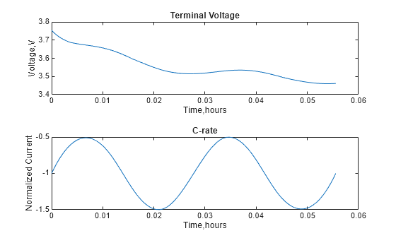
Plot the resulting terminal voltage and the normalized current (C-rate) at all solution times, specified in hours.
figure
tiledlayout(2,1)
nexttile
plot(R.SolutionTimes./3600,R.TerminalVoltage)
xlabel("Time,hours")
ylabel("Voltage,V")
title("Terminal Voltage")
nexttile
plot(R.SolutionTimes./3600,R.NormalizedCurrent)
xlabel("Time,hours")
ylabel("Normalized Current")
title("C-rate")
Battery Charging
Specify the state of charge (SoC) as 0.05 to indicate that the battery is at 5% charge.
model.InitialConditions.StateOfCharge = 0.05;
Specify the electrolyte concentration.
model.InitialConditions.ElectrolyteConcentration = 1000;
Specify the normalized current as a constant for charging.
model.CyclingStep.NormalizedCurrent = 2;
Solve the model.
R = solve(model);
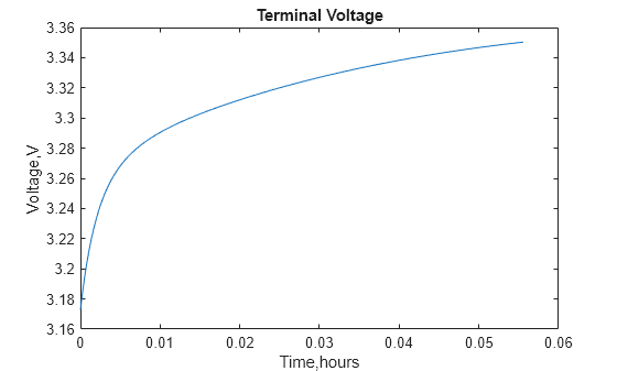
Plot the resulting terminal voltage at all solution times, specified in hours.
figure
plot(R.SolutionTimes./3600,R.TerminalVoltage)
xlabel("Time,hours")
ylabel("Voltage,V")
title("Terminal Voltage")