ModalThermalResults
Description
A ModalThermalResults object contains the eigenvalues and
eigenvector matrix of a thermal analysis problem, and average of snapshots used for proper
orthogonal decomposition (POD).
Creation
Solve a modal thermal problem using the solve function. This function returns a modal thermal solution as a ModalThermalResults object.
Properties
Examples
Solve a transient thermal problem by first obtaining mode shapes for a particular decay range and then using the modal superposition method.
Modal Decomposition
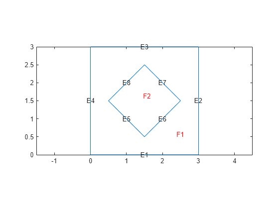
Create a geometry representing a square plate with a diamond-shaped region in its center.
SQ1 = [3; 4; 0; 3; 3; 0; 0; 0; 3; 3];
D1 = [2; 4; 0.5; 1.5; 2.5; 1.5; 1.5; 0.5; 1.5; 2.5];
gd = [SQ1 D1];
sf = 'SQ1+D1';
ns = char('SQ1','D1');
ns = ns';
g = decsg(gd,sf,ns);
pdegplot(g,EdgeLabels="on",FaceLabels="on")
xlim([-1.5 4.5])
ylim([-0.5 3.5])
axis equal
Create an femodel object for modal thermal analysis and include the geometry.
model = femodel(AnalysisType="thermalModal", ...
                Geometry=g);
For the square region, assign these thermal properties:
Thermal conductivity is .
Mass density is .
Specific heat is .
model.MaterialProperties(1) = ...
    materialProperties(ThermalConductivity=10, ...
                       MassDensity=2, ...
                       SpecificHeat=0.1);
For the diamond region, assign these thermal properties:
Thermal conductivity is .
Mass density is .
Specific heat is .
model.MaterialProperties(2) = ...
    materialProperties(ThermalConductivity=2, ...
                       MassDensity=1, ...
                       SpecificHeat=0.1);
Assume that the diamond-shaped region is a heat source with a density of .
model.FaceLoad(2) = faceLoad(Heat=4);
Apply a constant temperature of 0 °C to the sides of the square plate.
model.EdgeBC(1:4) = edgeBC(Temperature=0);
Set the initial temperature to 0 °C.
model.FaceIC = faceIC(Temperature=0);
Generate the mesh.
model = generateMesh(model);
Compute eigenmodes of the model in the decay range [100,10000] .
RModal = solve(model,DecayRange=[100,10000])
RModal =
  ModalThermalResults with properties:

    DecayRates: [164×1 double]
    ModeShapes: [1461×164 double]
      ModeType: "EigenModes"
          Mesh: [1×1 FEMesh]
Transient Analysis
Knowing the mode shapes, you can now use the modal superposition method to solve the transient thermal problem. First, switch the model analysis type to thermal transient.
model.AnalysisType = "thermalTransient";The dynamics for this problem are very fast. The temperature reaches a steady state in about 0.1 second. To capture the most active part of the dynamics, set the solution time to logspace(-2,-1,100). This command returns 100 logarithmically spaced solution times between 0.01 and 0.1.
tlist = logspace(-2,-1,10);
Solve the equation.
Rtransient = solve(model,tlist,ModalResults=RModal);
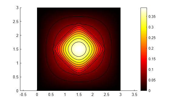
Plot the solution with isothermal lines by using a contour plot.
msh = Rtransient.Mesh
msh =
  FEMesh with properties:

             Nodes: [2×1461 double]
          Elements: [6×694 double]
    MaxElementSize: 0.1697
    MinElementSize: 0.0849
     MeshGradation: 1.5000
    GeometricOrder: 'quadratic'
T = Rtransient.Temperature;
pdeplot(msh,XYData=T(:,end),Contour="on", ...
                            ColorMap="hot")
axis equal
Obtain POD modes of a linear thermal problem using several instances of the transient solution (snapshots).
Create an femodel object for transient thermal analysis and include a unit square geometry in the model.
model = femodel(AnalysisType="thermalTransient", ...
                Geometry=@squareg);
Plot the geometry, displaying edge labels.
pdegplot(model.Geometry,EdgeLabels="on")
xlim([-1.1 1.1])
ylim([-1.1 1.1])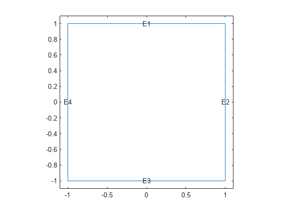
Specify the thermal conductivity, mass density, and specific heat of the material.
model.MaterialProperties = ...
    materialProperties(ThermalConductivity=400, ...
                       MassDensity=1300, ...
                       SpecificHeat=600);
Set the temperature on the right edge to 100.
model.EdgeBC(2) = edgeBC(Temperature=100);
Set an initial value of 0 for the temperature.
model.FaceIC = faceIC(Temperature=0);
Generate a mesh.
model = generateMesh(model);
Solve the model for three different values of heat source and collect snapshots.
tlist = 0:10:600;
snapShotIDs = [1:10 59 60 61];
Tmatrix = [];

heatVariation = [10000 15000 20000];
for q = heatVariation
    model.FaceLoad = faceLoad(Heat=q);
    results = solve(model,tlist);
    Tmatrix = [Tmatrix,results.Temperature(:,snapShotIDs)];
end
Switch the model analysis type to thermal modal.
model.AnalysisType = "thermalModal";Compute the POD modes.
RModal = solve(model,Snapshots=Tmatrix)
RModal =
  ModalThermalResults with properties:

          DecayRates: [6×1 double]
          ModeShapes: [1529×6 double]
    SnapshotsAverage: [1529×1 double]
            ModeType: "PODModes"
                Mesh: [1×1 FEMesh]
Version History
Introduced in R2022a