Vibration of Circular Membrane

This example shows how to calculate the vibration modes of a circular membrane.

The calculation of vibration modes requires the solution of the eigenvalue partial differential equation. This example compares the solution obtained by using the solvepdeeig solver from Partial Differential Toolbox™ and the eigs solver from MATLAB®. Eigenvalues calculated by solvepdeeig and eigs are practically identical, but in some cases one solver is more convenient than the other. For example, eigs is more convenient when calculating a specified number of eigenvalues in the vicinity of a particular target value. While solvepdeeig requires that a lower and upper bound surrounding this target, eigs requires only the target eigenvalue and the desired number of eigenvalues.

Create a PDE model.

model = createpde;

Create the circle geometry and include it in the model.

radius = 2;
g = decsg([1 0 0 radius]','C1',('C1')');

geometryFromEdges(model,g);

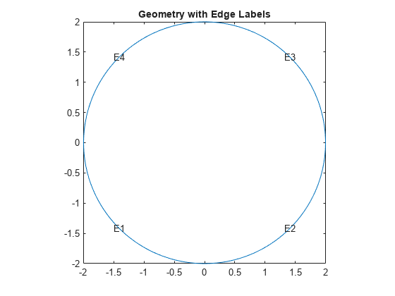
Plot the geometry with the edge labels.

figure
pdegplot(model,EdgeLabels="on")
axis equal
title("Geometry with Edge Labels")

Specify the coefficients.

c = 1e2;
a = 0;
f = 0;
d = 10;
specifyCoefficients(model,m=0,d=d,c=c,a=a,f=f);

Specify that the solution is zero at all four outer edges of the circle.

bOuter = applyBoundaryCondition(model,"dirichlet",Edge=(1:4),u=0);

Generate a mesh.

generateMesh(model,Hmax=0.2);

Use assembleFEMatrices to calculate the global finite element mass and stiffness matrices with boundary conditions imposed using the nullspace approach.

FEMatrices = assembleFEMatrices(model,"nullspace");
K = FEMatrices.Kc;
B = FEMatrices.B;
M = FEMatrices.M;

Solve the eigenvalue problem by using the eigs function.

sigma = 1e2; 
numberEigenvalues = 5;
[eigenvectorsEigs,eigenvaluesEigs] = eigs(K,M,numberEigenvalues,sigma);

Reshape the diagonal eigenvaluesEigs matrix into a vector.

eigenvaluesEigs = diag(eigenvaluesEigs);

Find the largest eigenvalue and its index in the eigenvalues vector.

[maxEigenvaluesEigs,maxIndex] = max(eigenvaluesEigs);

Add the constraint values to get the full eigenvector.

eigenvectorsEigs = B*eigenvectorsEigs;

Now, solve the same eigenvalue problem using solvepdeeig. Set the range for solvepdeeig to be slightly larger than the range from eigs.

r = [min(eigenvaluesEigs)*0.99 max(eigenvaluesEigs)*1.01];
result = solvepdeeig(model,r);
eigenvectorsPde = result.Eigenvectors;
eigenvaluesPde = result.Eigenvalues;

Compare the solutions.

eigenValueDiff = sort(eigenvaluesPde) - sort(eigenvaluesEigs);
fprintf(['Max difference in eigenvalues' ...
         ' from solvepdeeig and eigs: %e\n'], ...
  norm(eigenValueDiff,inf));

Max difference in eigenvalues from solvepdeeig and eigs: 2.842171e-13

Both functions calculate the same eigenvalues. For any eigenvalue, you can multiply the eigenvector by an arbitrary scalar. The eigs and solvepdeeig functions might choose a different arbitrary scalar for normalizing their eigenvectors.

h = figure;
h.Position = [1 1 2 1].*h.Position;
subplot(1,2,1)
axis equal
pdeplot(model,XYData=eigenvectorsEigs(:,maxIndex),Contour="on")
title(sprintf("eigs eigenvector,eigenvalue:%12.4e", ...
               eigenvaluesEigs(maxIndex)))
xlabel("x")
ylabel("y")
subplot(1,2,2)
axis equal
pdeplot(model,XYData=eigenvectorsPde(:,end),Contour="on")
title(sprintf("solvepdeeig eigenvector,eigenvalue:%12.4e", ...
               eigenvaluesPde(end)))
xlabel("x")
ylabel("y")