FPGA-Based Uniform Linear Array MVDR Beamformer
This example shows how to implement a minimum-variance distortionless-response (MVDR) beamformer suitable for hardware.
For more information on beamformers, see Conventional and Adaptive Beamformers.
MVDR Objective
The MVDR beamformer preserves the gain in the direction of arrival of a desired signal and attenuates interference from other directions [1], [2].
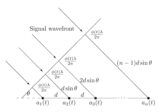
Given readings from a sensor array, such as the uniform linear array (ULA) in the following diagram, form data matrix  from samples of the array, where
  is an
is an  -by-1 column vector of readings from the array sampled at time
  , and
, and  is one row of matrix . Many more samples are taken than there are elements in the array. This results in the number of rows in being much greater than the number of columns. An estimate of the covariance matrix is
  , where
  is the Hermitian or complex-conjugate transpose of .
Compute the MVDR beamformer response by solving the following equation for  , where
  is a steering vector pointing in the direction of the desired signal.

The MVDR weight vector  is computed from and using the following equation, which normalizes to preserve the gain in the direction of arrival of the desired signal.

The MVDR system response is the inner product between the MVDR weight vector and a current sample from the sensor array .

HDL-Optimized MVDR
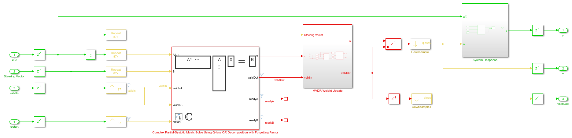
The three equations in the previous section are implemented by the three primary blocks in the following model. The rate changes give the matrix solve additional clock cycles to update before the next input sample. The number of clock cycles between a valid input and when the complex matrix solve block is ready is twice its input wordlength to allow time for CORDIC iterations, plus 15 cycles for internal delays.
load_system('MVDRBeamformerHDLOptimizedModel');
open_system('MVDRBeamformerHDLOptimizedModel/MVDR - HDL Optimized')
Instead of forming data matrix and computing the Cholesky factorization of covariance matrix , the upper-triangular matrix of the QR decomposition of is computed directly and updated as each data vector streams in from the sensor array. Because the data is updated indefinitely, a forgetting factor is applied after each factorization. To integrate with an equivalent of a matrix of  rows, the forgetting factor
  should be set to
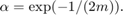
This example simulates the equivalent of a matrix with  rows, so the forgetting factor is set to 0.9983.
The Complex Partial-Systolic Matrix Solve Using Q-less QR Decomposition with Forgetting Factor block is implemented using the method found in [3]. The upper-triangular matrix  from the QR decomposition of is identical to the Cholesky factorization of except the signs of values on the diagonal. Solving the matrix equation
  by computing the Cholesky factorization of is not as efficient or as numerically sound as computing the QR decomposition of directly [4].
Run Model
Open and simulate the model.
open_system('MVDRBeamformerHDLOptimizedModel')
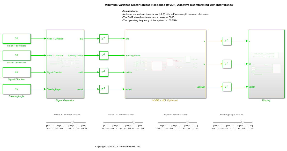
As the model is simulating, you can adjust the signal direction, steering angle and noise directions by dragging the sliders, or by editing the constant values.
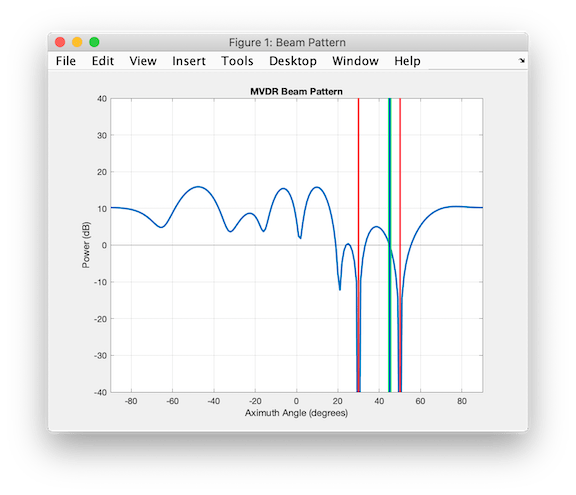
When the signal direction and steering angle are aligned as indicated by the blue and green lines, you can see that the beam pattern has a gain of 0 dB. The noise sources are nulled as indicated by the red lines.
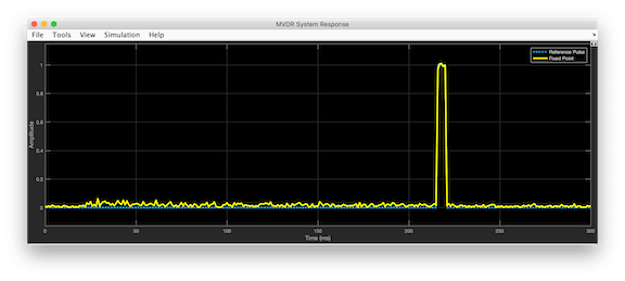
The desired pulse appears when the noise sources are nulled. This example simulates with the same latency as the hardware, so you can see the signal settle over time as the simulation starts and when the directions are changed.
Set Parameters
The parameters for the beamformer are set in the model workspace. You can modify the parameters by editing and running the setMVDRExampleModelWorkspace function.
References
[1] V. Behar et al. "Parameter Optimization of the adaptive MVDR QR-based beamformer for jamming and multipath supression in GPS/GLONASS receivers". In: Proc. 16th Saint Petersburg International Conference on Integrated Navigation systems. Saint Petersburg, Russia, May 2009, pp. 325--334.
[2] Jack Capon. "High-resolution frequency-wavenumber spectrum analysis". In: vol. 57. 1969, pp. 1408--1418.
[3] C.M. Rader. "VLSI Systolic Arrays for Adaptive Nulling". In: IEEE Signal Processing Magazine (July 1996), pp. 29--49.
[4] Charles F. Van Loan. Introduction to Scientific Computing: A Matrix-Vector Approach Using Matlab. Second edition. Prentice-Hall, 2000. isbn: 0-13-949157-0.