FPGA-Based Cell-Averaging Constant False Alarm Rate (CA-CFAR) Detector
This example shows how to design a CA-CFAR detector suitable for hardware.
To verify the implementation model is functionally correct, we compare the simulation output of the implementation model with the output of a CFAR based behavioral model using Phased Array System Toolbox™. The term deployment here implies designing a model that is suitable for implementation on a FPGA. The model is implementation ready and this will be verified in the example. The HDL workflow is designed in fixed-point.
The Phased Array System Toolbox provides the floating point behavioral model for the CFAR detector through the phased.CFARDetector System object™. This behavioral model is used to verify the results of the implementation model and the automatically generated HDL code as well.
Fixed-Point Designer™ provides data types and tools for developing fixed-point and single precision algorithms to optimize performance on an embedded hardware. Bit true simulations can be performed to observe the impact of limited range and precision without implementing the design in hardware.
This example uses HDL Coder™ to generate HDL Code from the developed Simulink® model and verifies the HDL Code using the HDL Verifier™. HDL Verifier is used to generate a cosimulation test bench model to verify the behavior of the automatically generated HDL Code. The test bench uses ModelSim® for cosimulation to verify the generated HDL code.
Algorithm Design
In a radar system, target detection is achieved by comparing the received signal power to a global threshold. If the received power is greater than the threshold, it marks the presence of a target else a target is said to be absent. This makes the choice of threshold a critical characteristic. The appropriate threshold value depends on maximizing the detection and minimizing the false alarm.
The threshold is chosen based on apriori knowledge (estimate) of the interferer power. The interferer power is affected by many external factors, hence, the variance will be a large value when measured globally. When the threshold is constant, the increase in interferer power can lead to an increase in false detections and at the same time, if the interferer power drops significantly, the target might not be detected.
The CFAR detector, as the name suggests, maintains the specified false alarm rate by means of an Adaptive Thresholding, wherein the threshold is calculated based on the locality of the Cell Under Test (CUT) and this defines the cell for which detection is required. The interference power of the neighboring cells is used to calculate the threshold for a CUT. The detection threshold is calculated as
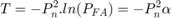
where,  is the Probability of False Alarm,
  is the Threshold Factor,
  is the Interference power level.
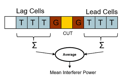
Cell-Averaging(CA) CFAR Detector In a CA CFAR, the lead and lag cells are used to calculate the interferer estimate. The number of lead cells are the same as that of the number of lag cells. CA-CFAR assumes that, the neighboring cells to the CUT contains the same interference statistic - Homogenous Interference and the target is present in only one CUT. To reinforce the second assumption, guard cells are placed immediately after the CUT.
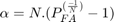
For a CA-CFAR with an independent and identically distributed (i.i.d) Gaussian interference (standard normal), the average noise power is just the mean of output of square law detector of all the training cells, which is

Here  is the signal from the i-th training cell. For a given Probability of False Alarm, the threshold factor can be calculated as,
The training cell and guard cell along with the CUT is called as the CFAR Window. The following figure shows a representation of a CFAR Window.
Implementation Model
The implementation model is designed using the HDL Coder compatible blocks from the Simulink HDL Coder library. For this example, we have chosen the following values for the parameters:
No. of Training Cells = 50
No. of Guard Cells = 2
Probability of False Alarm = 0.005
Total No. of Cells = 1000
The following command is used to open the Simulink model.
modelname = 'SimulinkCFARHDLWorkflowExample';
open_system(modelname);
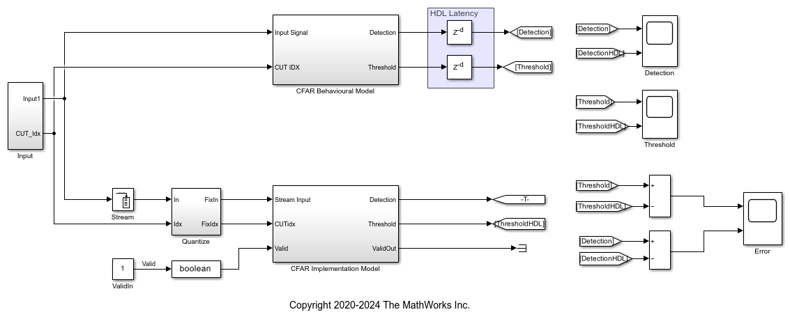
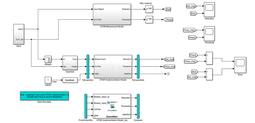
The Simulink model consists of two branches from the input block. The top branch is the behavioral model with floating point operations of the phased.CFARdetector System object. The bottom branch is the functional equivalent implementation model with fixed-point version.
The input to the behavioral model is a (NCell x 1) 1000x1 matrix. The input is passed through the Square-Law sub-system which performs the square-law operation which is then forwarded into the CFAR Detector behavioral model.
The input to the implementation model is provided via buffer which converts a multi-dimensional signal into single dimensional data stream for a deployable model. The input data type is then converted to fixed-point using the Quantize block. The fixed-point has a word-length of 24 bits and a fraction length of 12 bits. The tradeoff between different fixed-point setting with resource utilization and accuracy is discussed later in this example. The input is then passed on to the CFAR implementation model sub-system which performs the CFAR Detection.
The output of the CFAR Detector behavioral model is passed through a delay of 125 cycles to compensate the delay for the output of the implementation model.
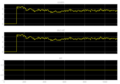
The scope block plots the threshold and detection outputs of the behavioral model and implementation model. In addition, the error between the threshold of implementation model and behavioral model, and the error between the detection of implementation model and behavioral model is also calculated and plotted.
The implementation model contains the following sub-systems:
Square-Law HDL
Alpha HDL
CFAR Core HDL
Validate
Square-Law HDL
The following command is used to open the Square-Law HDL subsystem model
open_system([modelname '/CFAR Implementation Model/Square Law HDL']);

The model computes the square-law envelope of the complex input signal.
For the implementation model the square-law is designed as a deployable model, with additional pipelining registers. This model is implemented using adders and multipliers which account for a latency of 6 cycles.
Alpha HDL
The following command is used to open the Alpha HDL subsystem model
open_system([modelname '/CFAR Implementation Model/Alpha HDL']);
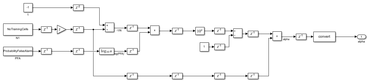
The Alpha HDL block utilizes the No. of Training Cells and Probability of False Alarm value to calculate the threshold factor ( ).
).
This subsystem uses Math HDL blocks and works in single precision for the native floating-point division operation which is then converted to fixed-point at the output. This block accounts for a pipeline latency of 7 Cycles.
CFAR Core HDL
%The following command is used to open the CFAR Core subsystem model
open_system([modelname '/CFAR Implementation Model/CFAR Core']);
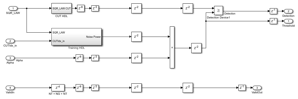
This subsystem extracts the training cells from the input stream and calculates the noise power. The noise power is then multiplied by alpha to generate the threshold which is later used in the detection process. There are two outputs from this block, namely, threshold and detection.
The threshold is the direct output of the product block whereas the detection output is provided through a comparator block which compares the threshold and signal value of CUT and returns true if the CUT signal is greater than the threshold.
This subsystem accounts for an input streaming delay of 102 (2*NumberTrainingCells + NoGuardCells) clock cycles with an additional pipelining latency of another 23 cycles. The total HDL latency is 125 cycles.
This block contains the following subsystems:
Training HDL
CUT HDL
Training HDL
The following command is used to open the Training HDL subsystem model.
open_system([modelname '/CFAR Implementation Model/CFAR Core/Training HDL']);
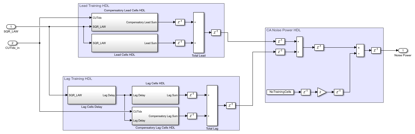
The lead training HDL subsystem extracts the lead cells of the CUT and performs a running sum. At the same time the lag training HDL subsystem pulls out the lag cells of the CUT and performs a running sum with a latency of 8 cycles each. The implementation of the lead training HDL and lag training HDL is very much analogous to a moving average filter the difference is that instead of the average we use the sum of window elements.
The CA noise power HDL subsystem sums up the lead power value and the lag power value and estimates the average noise power by dividing the sum by 100 (2*NoTrainingCells). This blocks accounts for a delay of 3 clock cycles.
The output of the training HDL subsystem is the noise power which is used to calculate the threshold.
CUT HDL
The following command is used to open the CUT HDL subsystem model
open_system([modelname '/CFAR Implementation Model/CFAR Core/CUT HDL']);
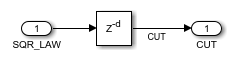
This subsystem uses a single delay block with a delay of 102 (2*NumberTrainingCells + NoGuardCells) cycles to time-align the CUT with the generated threshold value from the training HDL block. The above delay is the minimum delay required before which the CFAR Detector can detect the target at the first cell.
Validate
The following command is used to open the validate subsystem model
open_system([modelname '/CFAR Implementation Model/Validate']);

The valid input along with the latency is used to check the validity of the output. When the output is not valid this subsystem sends zero to the output.
Comparing the Results of Implementation Model to the Behavioral Model
The model can be simulated by clicking the Play button or using the sim command as shown below,
sim(modelname);
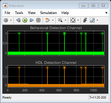
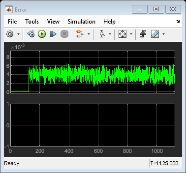

The Scope blocks are used to compare the output of implementation and behavioral model. The scope displays the detection and threshold from both the behavioral and implementation model and an additional scope displays the calculated the error.
The implementation model has a data streaming latency of 102 cycles and pipelining latency of 23 cycles. This in total accounts for an overall latency of 125 cycles. To time align the behavioral model with the implementation model we use an additional delay of 125 to the output of behavioral model.
With the 24 bit fixed-point of fraction length 12 bits, we have an error bounded by approximately 0.006 between the behavioral model and the implementation model threshold. Since the detection is Boolean we have no significant error in the detection output.
Code Generation and Verification
This section shows how to generate HDL code for the implementation model. It also shows how to verify that the generated code is functionally correct. The behavioral model provides the reference values to validate the output from HDL model.
If you start with a new Simulink model, call the hdlsetup function on the model to configure it for HDL code generation.
Model Settings
After the fixed-point implementation is verified and the implementation model produces the same results as your floating-point behavioral model, you can generate HDL code and test bench. For code generation and test bench, set the HDL Code Generation parameters in the Configuration Parameters dialog. The following parameters in Model Settings are set under HDL Code Generation:
Target: Xilinx Vivado synthesis tool; Virtex7 family; Device xc7vx485t; package ffg1761, speed -1; and target frequency of 300 MHz.
Optimization: Clear all optimizations
Global Settings: Set the Reset type to Asynchronous
Test Bench: Select HDL test bench and Co-simulation model
HDL Code Verification via Cosimulation
After the model is set up, use HDL Workflow Advisor to generate HDL code and a cosimulation test bench to test the model. To open HDL Workflow Advisor right-click on the CFAR Implementation model subsystem, then in the HDL Coder app section, click the HDL Workflow Advisor button. Instead of using HDL Workflow Advisor you can optionally call these commands to generate HDL code and test bench from the command line. makehdl([modelname '/CFAR Implementation Model']); % Generate HDL code makehdltb([modelname '/CFAR Implementation Model']); % Generate Cosimulation test bench
Since all the optimizations are cleared we do not have to add extra delays to the behavioral output other than the HDL latency previously added. All the critical paths are manually pipelined in the implementation model, so no additional optimizations are needed.
When you generate the test bench, the tool creates a new Simulink model in your working directory named gm_<modelname>_mq. The model contains a ModelSim Simulator block and looks like this:
To open the test bench model, use this command. modelname = ['gm_',modelname,'_mq']; open_system(modelname);
The model will open the ModelSim HDL simulator and run the cosimulation model to display the simulation results. To run the test bench, click the Play button on the top of the Simulink canvas or use the command window.
sim(modelname);
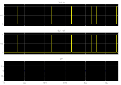
The Simulink test bench model populates the QuestaSim® window with the HDL model's Signal and Time Scopes in Simulink.

The Simulink scope shows detection output and threshold output for both the cosimulation and Design Under Test (DUT) as well as the error between them. The Compare subsystem in the test bench model contains scopes that compare the results of the cosimulation. The Compare subsystem is at the output of the CFAR_HDL_mq subsystem.
Fixed-Point Word Length and Fraction Length Tradeoffs
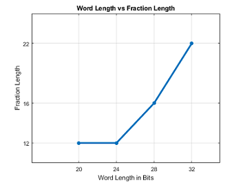
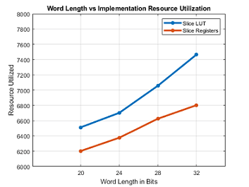
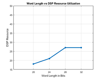
For this example a fixed-point word length of 24 bits and a fraction length of 12 bits are used for simulation and implementation. These figures show how choosing a longer fraction length would increase precision (reduces the Error) but also increases resource utilization.
This plot shows fraction length associated with chosen word length.
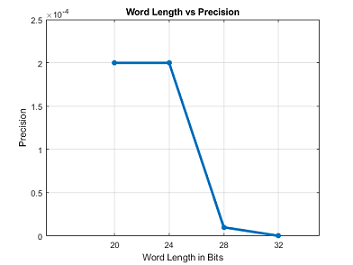
The next plot shows the precision with respect to chosen word length.
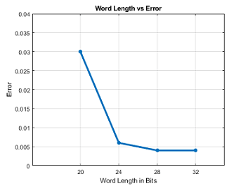
The next plot shows the Error with respect to chosen word length (Precision)
These plots show the LUT/Registers/DSP Utilization with respect to chosen word length.
Summary
This example demonstrated how to design a Simulink model for a Cell Averaging Constant False Alarm Rate(CA CFAR) Detector, and verify the results against behavioral code from the Phased Array System Toolbox. The model uses blocks that support HDL code generation. This example showed how to automatically generate HDL code for a fixed-point equivalent algorithm and verify the generated code in Simulink. The tool generates HDL code and a cosimulation test bench for the Simulink subsystem. This example showed how to setup and launch ModelSim to cosimulate the HDL code and compare its output to the output generated by the HDL implementation model.