High Resolution Direction of Arrival Estimation

Modeling the Received Array Signals

Define a uniform linear array (ULA) composed of 10 isotropic antennas. The array element spacing is 0.5 meters.

N = 10;
ula = phased.ULA('NumElements',N,'ElementSpacing',0.5)

ula = 
  phased.ULA with properties:

           Element: [1x1 phased.IsotropicAntennaElement]
       NumElements: 10
    ElementSpacing: 0.5000
         ArrayAxis: 'y'
             Taper: 1

Simulate the array output for two incident signals. Both signals are incident from 90° in azimuth. Their elevation angles are 73° and 68° respectively. In this example, we assume that these two directions are unknown and need to be estimated. Simulate the baseband received signal at the array demodulated from an operating frequency of 300 MHz.

fc = 300e6;                               % Operating frequency
fs = 8192;                                % Sampling frequency
lambda = physconst('LightSpeed')/fc;      % Wavelength
pos = getElementPosition(ula)/lambda;     % Element position in wavelengths
ang1 = [90;73]; ang2 = [90;68];           % Direction of the signals
angs = [ang1 ang2];
Nsamp = 1024;                             % Number of snapshots
noisePwr = 0.01;                          % Noise power

rs = rng(2012);                           % Set random number generator
signal = sensorsig(pos,Nsamp,angs,noisePwr);

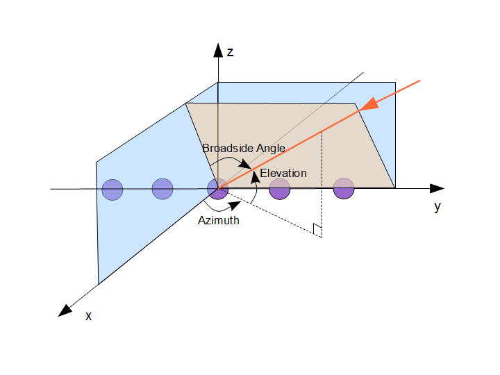
Because a ULA is symmetric around its axis, a DOA algorithm cannot uniquely determine azimuth and elevation. Therefore, the results returned by these high-resolution DOA estimators are in the form of broadside angles. An illustration of broadside angles can be found in the following figure.

Calculate the broadside angles corresponding to the two incident angles.

ang_true = az2broadside(angs(1,:),angs(2,:))

ang_true = 1×2

   17.0000   22.0000

The broadside angles are 17° and 22°.

Estimating the Direction of Arrival (DOA)

Assume that we know a priori that there are two sources. To estimate the DOA, use the root-MUSIC technique. Construct a DOA estimator using the root-MUSIC algorithm.

rootmusicangle = phased.RootMUSICEstimator('SensorArray',ula,...
            'OperatingFrequency',fc,...
            'NumSignalsSource','Property','NumSignals',2)

rootmusicangle = 
  phased.RootMUSICEstimator with properties:

                 SensorArray: [1x1 phased.ULA]
            PropagationSpeed: 299792458
          OperatingFrequency: 300000000
            NumSignalsSource: 'Property'
                  NumSignals: 2
    ForwardBackwardAveraging: false
            SpatialSmoothing: 0

Because the array response vector of a ULA is conjugate symmetric, we can use forward-backward (FB) averaging to perform computations with real matrices and reduce computational complexity. FB-based estimators also have a lower variance and reduce the correlation between signals.

To apply forward-backward averaging, set the ForwardBackwardAveraging property of the root-MUSIC DOA estimator to true. In this case, the root-MUSIC algorithm is also called the unitary root-MUSIC algorithm.

rootmusicangle.ForwardBackwardAveraging = true;

Perform the DOA estimation:

ang = rootmusicangle(signal)

ang = 1×2

   16.9960   21.9964

We can also use an ESPRIT DOA estimator. As in the case of root-MUSIC, set the ForwardBackwardAveraging property to true. This algorithm is also called unitary ESPRIT.

espritangle = phased.ESPRITEstimator('SensorArray',ula,...
             'OperatingFrequency',fc,'ForwardBackwardAveraging',true,...
             'NumSignalsSource','Property','NumSignals',2)

espritangle = 
  phased.ESPRITEstimator with properties:

                 SensorArray: [1x1 phased.ULA]
            PropagationSpeed: 299792458
          OperatingFrequency: 300000000
            NumSignalsSource: 'Property'
                  NumSignals: 2
            SpatialSmoothing: 0
                      Method: 'TLS'
    ForwardBackwardAveraging: true
                RowWeighting: 1

ang = espritangle(signal)

ang = 1×2

   21.9988   16.9748

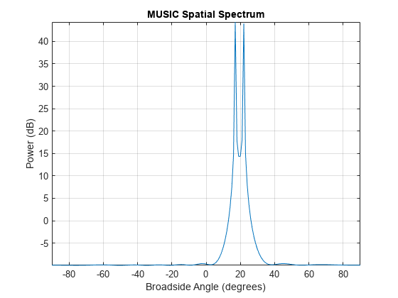
Finally, use the MUSIC DOA estimator. MUSIC also supports forward-backward averaging. Unlike ESPRIT and root-MUSIC, MUSIC computes a spatial spectrum for specified broadside scan angles. Directions of arrival correspond to peaks in the MUSIC spatial spectrum.

musicangle = phased.MUSICEstimator('SensorArray',ula,...
             'OperatingFrequency',fc,'ForwardBackwardAveraging',true,...
             'NumSignalsSource','Property','NumSignals',2,...
             'DOAOutputPort',true)

musicangle = 
  phased.MUSICEstimator with properties:

                 SensorArray: [1x1 phased.ULA]
            PropagationSpeed: 299792458
          OperatingFrequency: 300000000
    ForwardBackwardAveraging: true
            SpatialSmoothing: 0
                  ScanAngles: [-90 -89 -88 -87 -86 -85 -84 -83 -82 -81 -80 -79 -78 -77 -76 -75 -74 -73 -72 -71 -70 -69 -68 -67 -66 -65 -64 -63 -62 -61 -60 -59 -58 -57 -56 -55 -54 -53 -52 -51 -50 -49 -48 -47 -46 -45 -44 -43 -42 -41 -40 ... ] (1x181 double)
               DOAOutputPort: true
                  NumSignals: 2
            NumSignalsSource: 'Property'

[~,ang] = musicangle(signal)  

ang = 1×2

    17    22

plotSpectrum(musicangle)

Directions of arrival for MUSIC are limited to the scan angles in the ScanAngles property. Because the true directions of arrival in this example coincide with the search angles in ScanAngles, MUSIC provides precise DOA angle estimates. In practice, root-MUSIC provides superior resolution to MUSIC. However, the MUSIC algorithm can also be used for DOA estimation in both azimuth and elevation using a 2-D array. See Direction of Arrival Estimation with Beamscan, MVDR, and MUSIC.

Estimating the Number of Signal Sources

In practice, you generally do not know the number of signal sources, and need to estimate the number of sources from the received signal. You can estimate the number of signal sources by specifying 'Auto' for the NumSignalsSource property and choosing either 'AIC' or 'MDL' for the NumSignalsMethod property. For AIC, the Akaike information criterion (AIC) is used, and for MDL, the minimum description length (MDL) criterion is used.

Before you can set NumSignalsSource, you must release the DOA object because it is locked to improve efficiency during processing.

release(espritangle);
espritangle.NumSignalsSource = 'Auto';
espritangle.NumSignalsMethod = 'AIC';
ang = espritangle(signal)

ang = 1×2

   21.9988   16.9748

Reducing Computational Complexity

In addition to forward-backward averaging, other methods can reduce computational complexity. One of these approaches is to solve an equivalent problem with reduced dimensions in beamspace. While the ESPRIT algorithm performs the eigenvalue decomposition (EVD) of a 10x10 real matrix in our example, the beamspace version can reduce the problem to the EVD of a 3x3 real matrix. This technique uses a priori knowledge of the sector where the signals are located to position the center of the beam fan. In this example, point the beam fan to 20° in azimuth.

bsespritangle = phased.BeamspaceESPRITEstimator('SensorArray',ula,...
               'OperatingFrequency',fc,...
               'NumBeamsSource','Property','NumBeams',3,...
               'BeamFanCenter',20);
ang = bsespritangle(signal)

ang = 1×2

   21.9875   16.9943

Another technique is the root-weighted subspace fitting (WSF) algorithm. This algorithm is iterative and the most demanding in terms of computational complexity. You can set the maximum number of iterations by specifying the MaximumIterationCount property to maintain the cost below a specific limit.

rootwsfangle = phased.RootWSFEstimator('SensorArray',ula,...
          'OperatingFrequency',fc,'MaximumIterationCount',2);
ang = rootwsfangle(signal)

ang = 1×2

   16.9961   21.9962

Optimizing Performance

In addition to FB averaging, you can use row weighting to improve the statistical performance of the element-space ESPRIT estimator. Row weighting is a technique that applies different weights to the rows of the signal subspace matrix. The row weighting parameter determines the maximum weight. In most cases, it is chosen to be as large as possible. However, its value can never be greater than (N-1)/2, where N is the number of elements of the array.

release(espritangle);
espritangle.RowWeighting = 4

espritangle = 
  phased.ESPRITEstimator with properties:

                 SensorArray: [1x1 phased.ULA]
            PropagationSpeed: 299792458
          OperatingFrequency: 300000000
            NumSignalsSource: 'Auto'
            NumSignalsMethod: 'AIC'
            SpatialSmoothing: 0
                      Method: 'TLS'
    ForwardBackwardAveraging: true
                RowWeighting: 4

ang = espritangle(signal)

ang = 1×2

   21.9884   17.0003

Estimating Coherent Sources in Multipath Environments

If several sources are correlated or coherent (as in multipath environments), the spatial covariance matrix becomes rank deficient and subspace-based DOA estimation methods may fail. To show this, model a received signal composed of 4 narrowband components. Assume that 2 of the first 3 signals are multipath reflections of the first source, having magnitudes equal to 1/4 and 1/2 that of the first source, respectively.

scov = eye(4);
magratio = [1;0.25;0.5];
scov(1:3,1:3) = magratio*magratio';

All signals are incident at 0° elevation, with azimuth incident angles of -23°, 0°, 12°, and 40°.

% Incident azimuth
az_ang = [-23 0 12 40];

% When the elevation is zero, the azimuth within [-90 90] is the same as
% the broadside angle.
el_ang = zeros(1,4);

% The received signals
signal = sensorsig(pos,Nsamp,[az_ang; el_ang],noisePwr,scov);
rng(rs);  % Restore random number generator

Compare the performance of the DOA algorithm when sources are coherent. To simplify the example, run only one trial per algorithm. Given the high SNR, the results will be a good indicator of estimation accuracy.

First, verify that the AIC criterion underestimates the number of sources, causing the unitary ESPRIT algorithm to give incorrect estimates. The AIC estimates the number of sources as two because three sources are correlated.

release(espritangle);
espritangle.NumSignalsSource = 'Auto';
espritangle.NumSignalsMethod = 'AIC';
ang = espritangle(signal)

ang = 1×2

  -15.3535   40.0024

The root-WSF algorithm is robust in the context of correlated signals. With the correct number of sources as an input, the algorithm correctly estimates the directions of arrival.

release(rootwsfangle);
rootwsfangle.NumSignalsSource = 'Property';
rootwsfangle.NumSignals = 4;
ang = rootwsfangle(signal)

ang = 1×4

   40.0016  -22.9919   12.0693    0.0737

ESPRIT, root-MUSIC, and MUSIC, however, fail to estimate the correct directions of arrival, even if we specify the number of sources and use the unitary implementations.

release(rootmusicangle);
rootmusicangle.NumSignalsSource = 'Property';
rootmusicangle.NumSignals = 4;
rootmusicangle.ForwardBackwardAveraging = true;
ang = rootmusicangle(signal)

ang = 1×4

   40.0077  -22.8313    4.4976  -11.9038

You can apply spatial smoothing to estimate the DOAs of correlated signals. Using spatial smoothing, however, decreases the effective aperture of the array. Therefore, the variance of the estimators increases because the subarrays are smaller than the original array.

release(rootmusicangle);
Nr = 2;    % Number of multipath reflections 
rootmusicangle.SpatialSmoothing = Nr

rootmusicangle = 
  phased.RootMUSICEstimator with properties:

                 SensorArray: [1x1 phased.ULA]
            PropagationSpeed: 299792458
          OperatingFrequency: 300000000
            NumSignalsSource: 'Property'
                  NumSignals: 4
    ForwardBackwardAveraging: true
            SpatialSmoothing: 2

ang = rootmusicangle(signal)

ang = 1×4

   40.0010  -22.9959   12.1376    0.1843

Comparison of DOA Algorithms

In summary, ESPRIT, MUSIC, root-MUSIC, and root-WSF are important DOA algorithms that provide good performance and reasonable computational complexity for ULAs. Unitary ESPRIT, unitary root-MUSIC, and beamspace unitary ESPRIT provide ways to significantly reduce the computational cost of the estimators, while also improving their performance. root-WSF is particularly attractive in the context of correlated sources because, contrary to the other methods, it does not require spatial smoothing to properly estimate the DOAs when the number of sources is known.